How to Calculate the Duration Between Two Times in Google Sheets
Basics
Apr 28, 2024
There’s one thing you’ve probably tried to do in your spreadsheets but couldn’t figure out – we’re talking about calculating the duration between two times in Google Sheets. Whether you're scheduling meetings, tracking your working hours, or planning your day, knowing how to do this can be a game-changer.
The best part? This is actually super easy to figure out and doesn’t require advanced Sheets knowledge or anything like that. The only thing you need to figure out is how to subtract time. Let’s dive in.
Time format in Google Sheets
Before diving into calculations, you need to know how Google Sheets interprets and displays time. Google Sheets uses a serial number system to represent time, where one day is equivalent to the number 1. That means that Google Sheets represents time as a fraction of a day.
For instance, 12:00 PM is represented as 0.5 since it's halfway through the day.
How to subtract time in Google Sheets?
Step 1: Enter in the time data
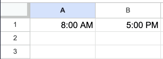
First you need to enter your start and end times into two separate cells. You’ll need to make sure that these times are in Google Sheets' recognized time format (hh:mm AM/PM or 24-hour format). For example, enter 8:00 AM in cell A1 and 5:00 PM in cell B1:
Step 2: Calculate the duration
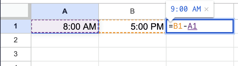
To calculate the duration, all you have to do is subtract the start time from the end time in a new cell. For example, in cell C1, enter the formula =B1-A1. This will give you the duration in the format of hours and minutes:
Step 3: Format the duration
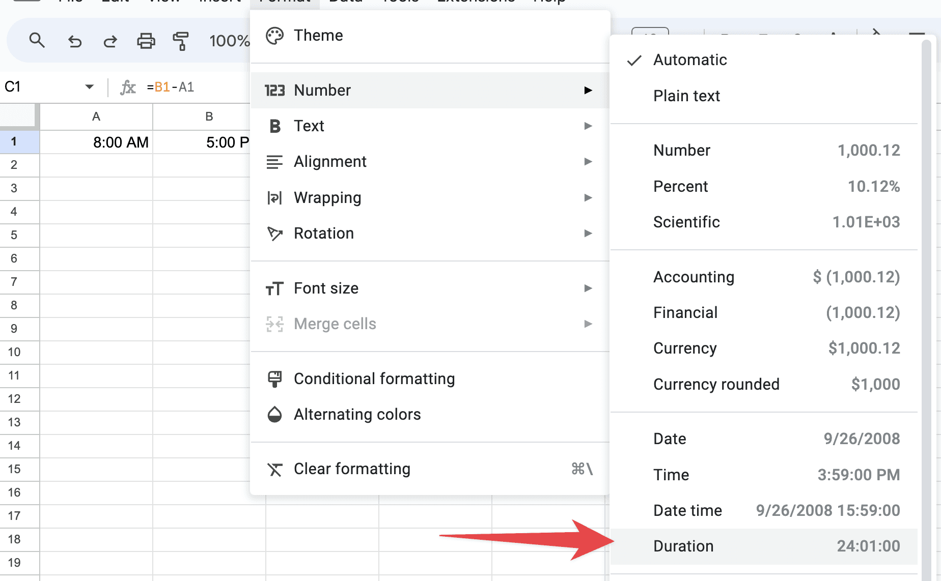
Sometimes Google Sheets will display the duration in an odd format, like a decimal number. To format this into a more readable time format you’ll just need to select the cell and go to Format → Number → Duration. This will convert your duration into a readable format, such as "9:00" for a 9-hour duration:
Other things to know
What if the duration crosses over from midnight?
If the end time that you’re looking at crosses midnight, just doing a straightforward subtraction will give you a negative number. You probably don’t want this.
There’s a pretty easy fix for this though. You can use the formula =MOD(B1-A1,1). The MOD function here helps to correctly calculate the time difference by considering the day roll-over.
How to calculate the total duration from a list?
You might be dealing with a situation where you have a whole bunch of start and end times to deal with. That’s totally fine though.
If you have a list of start and end times, you can calculate the total duration by using the SUM function in combination with individual duration calculations. For instance, if your times are in A1:B10, use =SUM(B1:B10-A1:A10) in a separate cell:
Advanced time calculations in Google Sheets
How to calculate business hours in Google Sheets?
If you’re looking to calculate durations within business hours, you’ll need a more complex formula that excludes the times that the business in question isn’t open, like non-business hours and weekends. This typically involves using the NETWORKDAYS function alongside some additional calculations to consider start and end times within each day.
How to calculate time differences in minutes and seconds?
To get the time difference in minutes or seconds, multiply the duration by 1440 (minutes in a day) or 86400 (seconds in a day) respectively. For example, =(B1-A1)*1440 will give you the difference in minutes.
Conditional time calculations
Sometimes, you might want to calculate duration only under certain conditions. For this, you can use the IF function combined with your time calculation formula. For example, =IF(B1>A1, B1-A1, “Time error”) to avoid negative durations.
Tips for accurate time calculations
How to calculate between different time zones?
If your time data involves different time zones then you’ll have to make sure that you are standardizing the times to a single zone before you run any calculations. Otherwise you’ll probably get an error.
One major challenge is variability. Different regions observe different time zones and might also follow Daylight Saving Time (DST), which is a whole other thing.
Another challenge is data integrity. Without standardization, time data can be misleading. For example, 9:00 AM in New York (EST) is actually 6:00 AM in Los Angeles (PST). Calculating the duration between these times without adjusting for the time zone will give you the wrong results.
You can avoid these headaches by standardizing your timezones:
Identify Time Zone for Each Data Point: First, determine the time zone of each time entry. You can do this by adding an additional column in your data specifying the time zone.
Choose a Standard Time Zone: Decide on a standard time zone to which all times will be converted. This could be the time zone of your business’s location, UTC (Coordinated Universal Time), or any other consistent reference.
Calculate Time Zone Offset: For each time entry, calculate the time difference between the local time zone and your standard time zone. For instance, if your standard time zone is EST and you have a time entry in PST, the offset will be -3 hours.
Adjust Times to Standard Time Zone: Use Google Sheets formulas to adjust each time entry to the standard time zone. If you’re working with a -3 hours offset, the formula would look like
=A1-(3/24), assuming your original time is in cell A1.Consider Daylight Saving Time (DST): If DST is observed in the time zone, make sure to adjust for it. This usually means an additional hour adjustment during specific months of the year.
For regular work with time zone data, consider automating the process using Google Sheets Scripts. Scripts can programmatically adjust times based on time zone and DST rules. This is especially useful when dealing with large datasets.
Be careful of the AM/PM format
When you’re entering times in the 12-hour format; always specify AM or PM to avoid confusion.
Consider using the 24-hour format (also known as military time) to eliminate any ambiguity. In this format, 8:00 AM is "08:00", and 8:00 PM is "20:00".
The good news is that you can format cells to display time correctly. In Google Sheets, you can set the cell format to 'Time' which will automatically prompt for AM/PM in the 12-hour format.
Use data validation for time inputs
To maintain consistency and avoid errors, use data validation (Data → Data Validation) to ensure that the cells designated for time inputs follow the correct time format.
For example you can set a data validation rule that checks for text length or specific characters (AM/PM) in the time entries.
About the Author

Kris Lachance
Managing Editor
Kris is the Managing Editor of Spreadsheet Secrets. He is a finance professional, writer and entrepreneur based in Canada.
How to Calculate the Duration Between Two Times in Google Sheets
Basics
Apr 28, 2024
There’s one thing you’ve probably tried to do in your spreadsheets but couldn’t figure out – we’re talking about calculating the duration between two times in Google Sheets. Whether you're scheduling meetings, tracking your working hours, or planning your day, knowing how to do this can be a game-changer.
The best part? This is actually super easy to figure out and doesn’t require advanced Sheets knowledge or anything like that. The only thing you need to figure out is how to subtract time. Let’s dive in.
Time format in Google Sheets
Before diving into calculations, you need to know how Google Sheets interprets and displays time. Google Sheets uses a serial number system to represent time, where one day is equivalent to the number 1. That means that Google Sheets represents time as a fraction of a day.
For instance, 12:00 PM is represented as 0.5 since it's halfway through the day.
How to subtract time in Google Sheets?
Step 1: Enter in the time data
First you need to enter your start and end times into two separate cells. You’ll need to make sure that these times are in Google Sheets' recognized time format (hh:mm AM/PM or 24-hour format). For example, enter 8:00 AM in cell A1 and 5:00 PM in cell B1:
Step 2: Calculate the duration
To calculate the duration, all you have to do is subtract the start time from the end time in a new cell. For example, in cell C1, enter the formula =B1-A1. This will give you the duration in the format of hours and minutes:
Step 3: Format the duration
Sometimes Google Sheets will display the duration in an odd format, like a decimal number. To format this into a more readable time format you’ll just need to select the cell and go to Format → Number → Duration. This will convert your duration into a readable format, such as "9:00" for a 9-hour duration:
Other things to know
What if the duration crosses over from midnight?
If the end time that you’re looking at crosses midnight, just doing a straightforward subtraction will give you a negative number. You probably don’t want this.
There’s a pretty easy fix for this though. You can use the formula =MOD(B1-A1,1). The MOD function here helps to correctly calculate the time difference by considering the day roll-over.
How to calculate the total duration from a list?
You might be dealing with a situation where you have a whole bunch of start and end times to deal with. That’s totally fine though.
If you have a list of start and end times, you can calculate the total duration by using the SUM function in combination with individual duration calculations. For instance, if your times are in A1:B10, use =SUM(B1:B10-A1:A10) in a separate cell:
Advanced time calculations in Google Sheets
How to calculate business hours in Google Sheets?
If you’re looking to calculate durations within business hours, you’ll need a more complex formula that excludes the times that the business in question isn’t open, like non-business hours and weekends. This typically involves using the NETWORKDAYS function alongside some additional calculations to consider start and end times within each day.
How to calculate time differences in minutes and seconds?
To get the time difference in minutes or seconds, multiply the duration by 1440 (minutes in a day) or 86400 (seconds in a day) respectively. For example, =(B1-A1)*1440 will give you the difference in minutes.
Conditional time calculations
Sometimes, you might want to calculate duration only under certain conditions. For this, you can use the IF function combined with your time calculation formula. For example, =IF(B1>A1, B1-A1, “Time error”) to avoid negative durations.
Tips for accurate time calculations
How to calculate between different time zones?
If your time data involves different time zones then you’ll have to make sure that you are standardizing the times to a single zone before you run any calculations. Otherwise you’ll probably get an error.
One major challenge is variability. Different regions observe different time zones and might also follow Daylight Saving Time (DST), which is a whole other thing.
Another challenge is data integrity. Without standardization, time data can be misleading. For example, 9:00 AM in New York (EST) is actually 6:00 AM in Los Angeles (PST). Calculating the duration between these times without adjusting for the time zone will give you the wrong results.
You can avoid these headaches by standardizing your timezones:
Identify Time Zone for Each Data Point: First, determine the time zone of each time entry. You can do this by adding an additional column in your data specifying the time zone.
Choose a Standard Time Zone: Decide on a standard time zone to which all times will be converted. This could be the time zone of your business’s location, UTC (Coordinated Universal Time), or any other consistent reference.
Calculate Time Zone Offset: For each time entry, calculate the time difference between the local time zone and your standard time zone. For instance, if your standard time zone is EST and you have a time entry in PST, the offset will be -3 hours.
Adjust Times to Standard Time Zone: Use Google Sheets formulas to adjust each time entry to the standard time zone. If you’re working with a -3 hours offset, the formula would look like
=A1-(3/24), assuming your original time is in cell A1.Consider Daylight Saving Time (DST): If DST is observed in the time zone, make sure to adjust for it. This usually means an additional hour adjustment during specific months of the year.
For regular work with time zone data, consider automating the process using Google Sheets Scripts. Scripts can programmatically adjust times based on time zone and DST rules. This is especially useful when dealing with large datasets.
Be careful of the AM/PM format
When you’re entering times in the 12-hour format; always specify AM or PM to avoid confusion.
Consider using the 24-hour format (also known as military time) to eliminate any ambiguity. In this format, 8:00 AM is "08:00", and 8:00 PM is "20:00".
The good news is that you can format cells to display time correctly. In Google Sheets, you can set the cell format to 'Time' which will automatically prompt for AM/PM in the 12-hour format.
Use data validation for time inputs
To maintain consistency and avoid errors, use data validation (Data → Data Validation) to ensure that the cells designated for time inputs follow the correct time format.
For example you can set a data validation rule that checks for text length or specific characters (AM/PM) in the time entries.
About the Author
Kris Lachance
Managing Editor
Kris is the Managing Editor of Spreadsheet Secrets. He is a finance professional, writer and entrepreneur based in Canada.

Spreadsheet Secrets
Helping you get better at all things spreadsheets. From learning functions to helpful tips and tricks. Microsoft Excel, Google Sheets, Apple Numbers, Office 365, whatever you use we can help you with.
Contact us here: ssheetsecrets@gmail.com
© 2024 Spreadsheet Secrets.
Spreadsheet Secrets
Helping you get better at all things spreadsheets. From learning functions to helpful tips and tricks. Microsoft Excel, Google Sheets, Apple Numbers, Office 365, whatever you use we can help you with.
Contact us here: ssheetsecrets@gmail.com
© 2024 Spreadsheet Secrets.
Spreadsheet Secrets
Helping you get better at all things spreadsheets. From learning functions to helpful tips and tricks. Microsoft Excel, Google Sheets, Apple Numbers, Office 365, whatever you use we can help you with.
Contact us here: ssheetsecrets@gmail.com
© 2024 Spreadsheet Secrets.