How to Freeze a Row in Google Sheets
Basics
Apr 19, 2024
If you want to work with a simple spreadsheet, Google Sheets is king. It’s a great app. But there’s a quirk that can be infuriating if you don’t know the right fix for it. We’re talking about when you want to scroll down your spreadsheet but you keep losing the header. It’s annoying to have to scroll back up each time you want to see what’s in the particular column you’re looking at.
Luckily there’s an easy fix for this: you can do what’s called “freezing” a row. This basically makes it so that you can create a fixed, static “header” at the top of your spreadsheet. Once you have frozen the row, the header will stay there no matter how far you scroll down. This post covers how to set that up and gives you a couple of other neat tricks for keeping your spreadsheet clean.
If you’ve ever asked yourself a question like “how do I pin a header in Google Sheets?” or “how do I make the header stay?” then keep reading.
What is freezing a row in Google Sheets?
In Google Sheets, freezing a row is a feature that lets you keep specific rows visible at the top of the sheet as you scroll down through the rest of your data. This comes in handy when you have a spreadsheet with headers or labels in the top row (or first few rows) that describe the data in the columns below. By freezing these rows, you keep them visible, making it easier to view and understand your data as you scroll through your sheet.
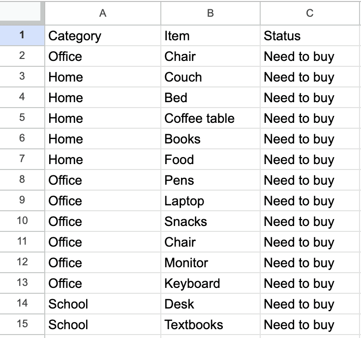
For example, if you have a spreadsheet where the first row contains column headers like "Category," "Item," "Status," etc., then freezing the first row will keep these headers in place at the top of the screen, even as you scroll down to view entries that are further down in your spreadsheet. This way, you don't lose track of what each column represents, which helps maintain context and improves readability.
Why freeze a row in Google Sheets?
The main reason you’d want to freeze a row in Google Sheets is to keep headers visible so that you can compare data and make it easier to navigate your sheet.
To use the example from above, let’s say you’re working on a spreadsheet and you have several columns, as well as rows. You’ll have to either scroll up and down the sheet in order to remember what’s in each column, or mentally remember what each column is supposed to contain. Both options aren’t ideal because they make navigation and data comparison harder for you to do. Working with data is already challenging! Why would you make it more challenging! Much better to make things easier and reduce the mental load of your tasks. You’ll be much more productive and way happier.
There are a couple of options to freeze a row - we’ll cover them below.
The easiest way to freeze: use your mouse
The easiest way to freeze a row (or several rows) is with your mouse.
First, open your Google Sheets document.
Then, one you have the document open, the first step is to decide exactly what row (or rows) you want to freeze. Here, we want to freeze the first row of the following sheet, since “Category,” “Item” and “Status” are meant to be column headers.
Now that we’ve identified which row we want to freeze, the next step is to actually freeze it using the mouse. This is super easy. All you have to do is move your mouse to that grey box that sits on top of the “1” row marker and to the left of the “A” in Column A:
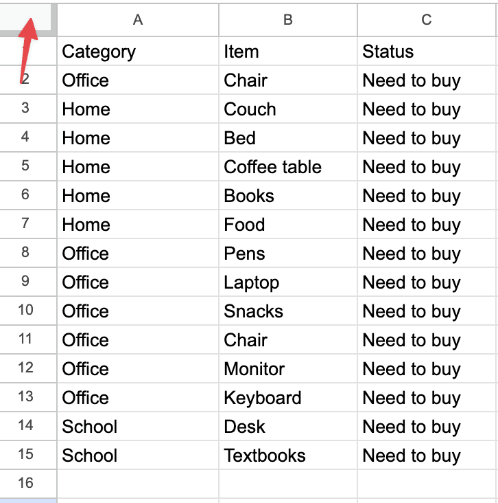
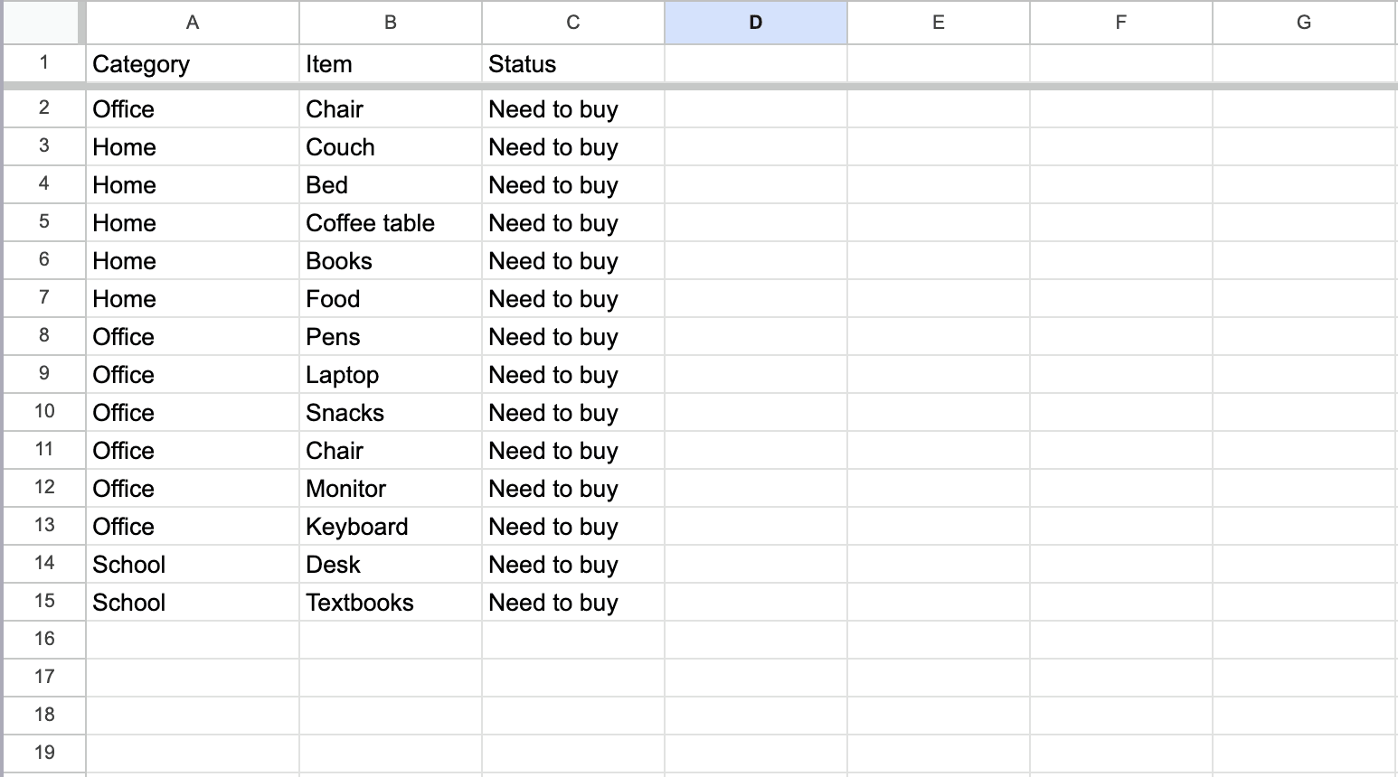
Now, hover over the bottom line of this box until you see that your mouse cursor turns into a hand icon. Once it does, simply drag the line down to cover the row(s) you want to freeze which, in our case, would just be the first row:

As you can see, the first row is pinned to the top of the sheet so that it stays in place as you scroll.
Freezing a row with the view menu
You can also freeze a row from the menu bar.
First, open your Google Sheets document.
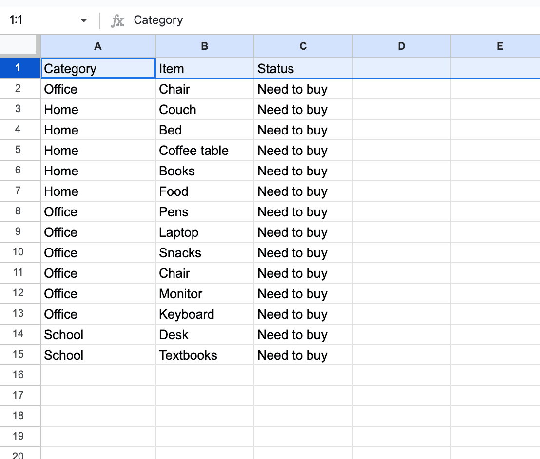
Then, once you have the document open, click on the row you want to freeze. Since we want to freeze the first row, this means we’ll want to click where it says the number “1”. This will highlight the entire row:
Then, go to the menu click on View > Freeze, and then select 1 row (or however many rows you want to freeze):
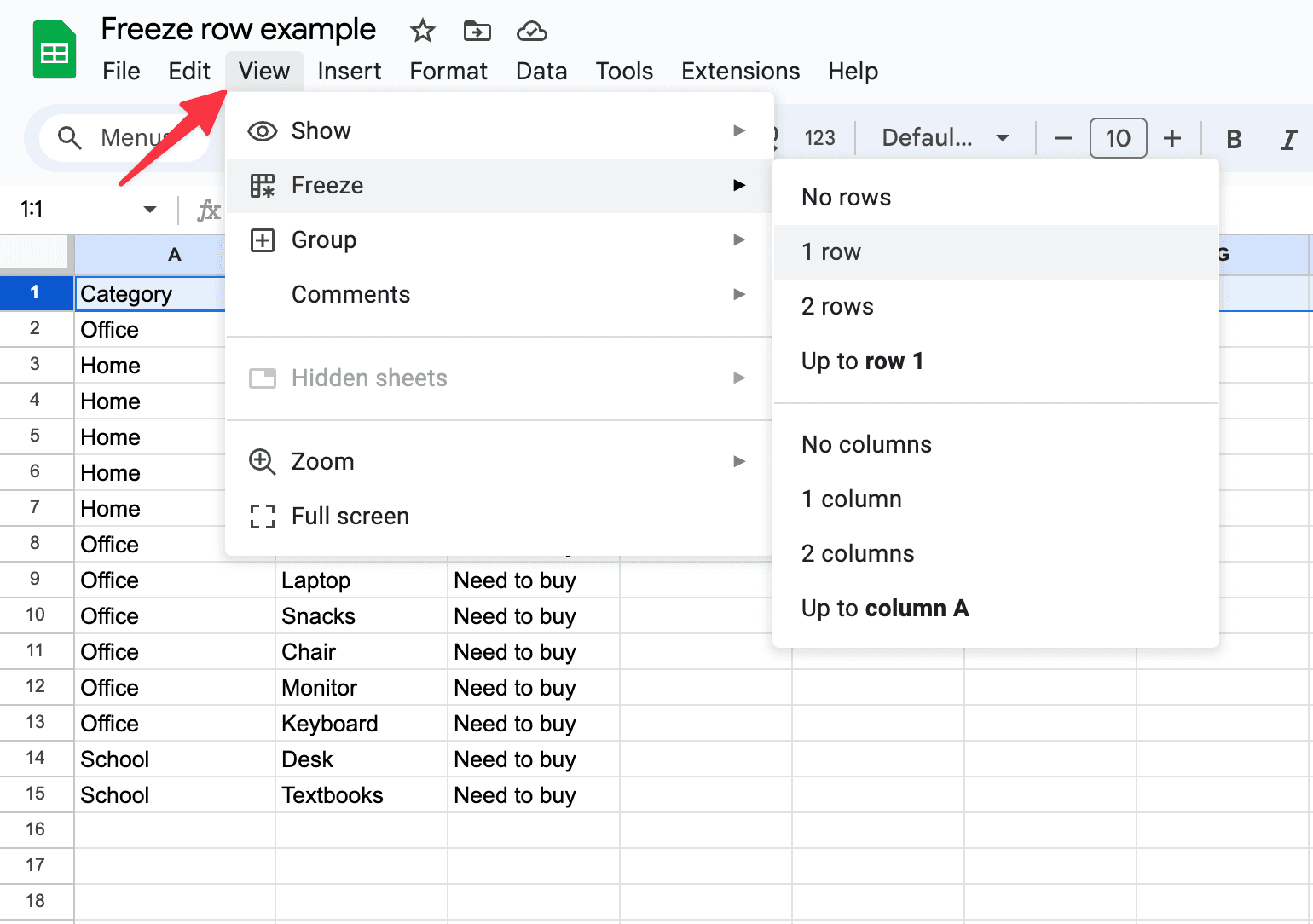
And voila, now the row is frozen!
How to unfreeze a row in Google Sheets
If you want to unfreeze a row that’s been frozen, that’s easy. Again, the best way is to use your mouse. Hover your mouse over the bar that marks the row you froze until you see the cursor turn into a hand icon. Once it does, simply click the row and drag it back to its original position:

How to freeze a column in Google Sheets
You can also freeze a column in Google Sheets. Simply hover your mouse over the grey box in the top left of the sheet and wait for the cursor to change into the hand icon. Once it does, drag the grey line on the right side of the box to cover the specific column (or columns) that you want to freeze.
This follows the same steps outlined above, but for columns.
How do you freeze panes in Google Sheets?
A pane is a section of your sheet that has already been frozen. You “freeze” a pane by freezing one or more rows and/or columns.
If you want to adjust a frozen pane ,simply drag the freeze handle (horizontal for rows, vertical for columns) to a new position. This will change the number of frozen rows or columns.
To remove frozen panes, go back to View > Freeze, and select No rows or No columns as appropriate. This will unfreeze the rows or columns, returning them to normal scrolling behavior.
About the Author

Harish Malhi
Managing Editor
Kris is the Managing Editor of Spreadsheet Secrets. He is a finance professional, writer and entrepreneur based in Canada.
How to Freeze a Row in Google Sheets
Basics
Apr 19, 2024
If you want to work with a simple spreadsheet, Google Sheets is king. It’s a great app. But there’s a quirk that can be infuriating if you don’t know the right fix for it. We’re talking about when you want to scroll down your spreadsheet but you keep losing the header. It’s annoying to have to scroll back up each time you want to see what’s in the particular column you’re looking at.
Luckily there’s an easy fix for this: you can do what’s called “freezing” a row. This basically makes it so that you can create a fixed, static “header” at the top of your spreadsheet. Once you have frozen the row, the header will stay there no matter how far you scroll down. This post covers how to set that up and gives you a couple of other neat tricks for keeping your spreadsheet clean.
If you’ve ever asked yourself a question like “how do I pin a header in Google Sheets?” or “how do I make the header stay?” then keep reading.
What is freezing a row in Google Sheets?
In Google Sheets, freezing a row is a feature that lets you keep specific rows visible at the top of the sheet as you scroll down through the rest of your data. This comes in handy when you have a spreadsheet with headers or labels in the top row (or first few rows) that describe the data in the columns below. By freezing these rows, you keep them visible, making it easier to view and understand your data as you scroll through your sheet.
For example, if you have a spreadsheet where the first row contains column headers like "Category," "Item," "Status," etc., then freezing the first row will keep these headers in place at the top of the screen, even as you scroll down to view entries that are further down in your spreadsheet. This way, you don't lose track of what each column represents, which helps maintain context and improves readability.
Why freeze a row in Google Sheets?
The main reason you’d want to freeze a row in Google Sheets is to keep headers visible so that you can compare data and make it easier to navigate your sheet.
To use the example from above, let’s say you’re working on a spreadsheet and you have several columns, as well as rows. You’ll have to either scroll up and down the sheet in order to remember what’s in each column, or mentally remember what each column is supposed to contain. Both options aren’t ideal because they make navigation and data comparison harder for you to do. Working with data is already challenging! Why would you make it more challenging! Much better to make things easier and reduce the mental load of your tasks. You’ll be much more productive and way happier.
There are a couple of options to freeze a row - we’ll cover them below.
The easiest way to freeze: use your mouse
The easiest way to freeze a row (or several rows) is with your mouse.
First, open your Google Sheets document.
Then, one you have the document open, the first step is to decide exactly what row (or rows) you want to freeze. Here, we want to freeze the first row of the following sheet, since “Category,” “Item” and “Status” are meant to be column headers.
Now that we’ve identified which row we want to freeze, the next step is to actually freeze it using the mouse. This is super easy. All you have to do is move your mouse to that grey box that sits on top of the “1” row marker and to the left of the “A” in Column A:
Now, hover over the bottom line of this box until you see that your mouse cursor turns into a hand icon. Once it does, simply drag the line down to cover the row(s) you want to freeze which, in our case, would just be the first row:
As you can see, the first row is pinned to the top of the sheet so that it stays in place as you scroll.
Freezing a row with the view menu
You can also freeze a row from the menu bar.
First, open your Google Sheets document.
Then, once you have the document open, click on the row you want to freeze. Since we want to freeze the first row, this means we’ll want to click where it says the number “1”. This will highlight the entire row:
Then, go to the menu click on View > Freeze, and then select 1 row (or however many rows you want to freeze):
And voila, now the row is frozen!
How to unfreeze a row in Google Sheets
If you want to unfreeze a row that’s been frozen, that’s easy. Again, the best way is to use your mouse. Hover your mouse over the bar that marks the row you froze until you see the cursor turn into a hand icon. Once it does, simply click the row and drag it back to its original position:
How to freeze a column in Google Sheets
You can also freeze a column in Google Sheets. Simply hover your mouse over the grey box in the top left of the sheet and wait for the cursor to change into the hand icon. Once it does, drag the grey line on the right side of the box to cover the specific column (or columns) that you want to freeze.
This follows the same steps outlined above, but for columns.
How do you freeze panes in Google Sheets?
A pane is a section of your sheet that has already been frozen. You “freeze” a pane by freezing one or more rows and/or columns.
If you want to adjust a frozen pane ,simply drag the freeze handle (horizontal for rows, vertical for columns) to a new position. This will change the number of frozen rows or columns.
To remove frozen panes, go back to View > Freeze, and select No rows or No columns as appropriate. This will unfreeze the rows or columns, returning them to normal scrolling behavior.
About the Author
Harish Malhi
Managing Editor
Kris is the Managing Editor of Spreadsheet Secrets. He is a finance professional, writer and entrepreneur based in Canada.

Spreadsheet Secrets
Helping you get better at all things spreadsheets. From learning functions to helpful tips and tricks. Microsoft Excel, Google Sheets, Apple Numbers, Office 365, whatever you use we can help you with.
Contact us here: ssheetsecrets@gmail.com
© 2024 Spreadsheet Secrets.
Spreadsheet Secrets
Helping you get better at all things spreadsheets. From learning functions to helpful tips and tricks. Microsoft Excel, Google Sheets, Apple Numbers, Office 365, whatever you use we can help you with.
Contact us here: ssheetsecrets@gmail.com
© 2024 Spreadsheet Secrets.
Spreadsheet Secrets
Helping you get better at all things spreadsheets. From learning functions to helpful tips and tricks. Microsoft Excel, Google Sheets, Apple Numbers, Office 365, whatever you use we can help you with.
Contact us here: ssheetsecrets@gmail.com
© 2024 Spreadsheet Secrets.