
How to Merge Cells in Google Sheets: A Guide
Basics
Apr 30, 2024
We love the fact that Google Sheets has all of these cells. It’s what helps make the data so clear. But what if you want to merge some of those cells together? That’s exactly what this guide covers.
What is cell merging in Google Sheets?
Merging cells involves combining two or more adjacent cells into a single cell. You’ll want to do this when you have data or titles across multiple columns or rows.
Be careful though. When you merge cells, only the upper-left cell will have its data intact. This means that if you have data in the other cells that are being merged, then the data in those cells will be deleted if you merge the cells.
How to merge cells in Google Sheets?
Step 1: Select which cells to merge
First, select the cells you want to merge. You can do this by clicking and dragging your mouse over the cells. For instance, if you want to merge a group of cells from A1 to C1, click on cell A1, hold down your mouse button, and drag across to C1:
Make sure that the cells are next to each other because Google Sheets doesn’t let you merge cells that aren’t next to each other.
Step 2: Merge the cells
Once you’ve selected the cells, it's time to perform the merge. Look for the 'Merge cells' icon in the Google Sheets toolbar. This icon looks like this:
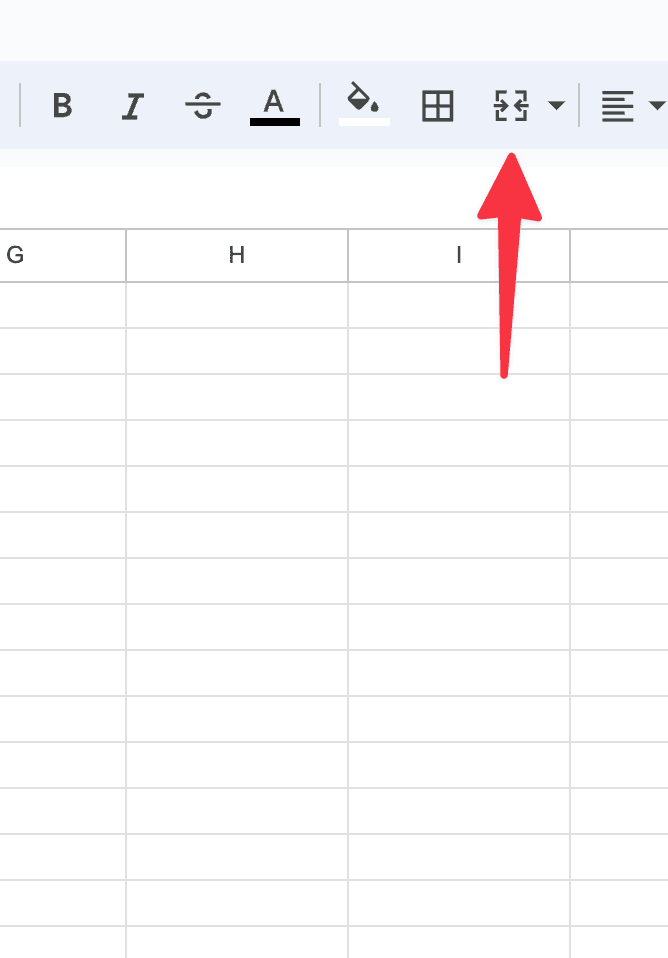
Click on the down arrow to the right of this icon and you’ll see a dropdown menu with three options: 'Merge all', 'Merge horizontally', and 'Merge vertically':
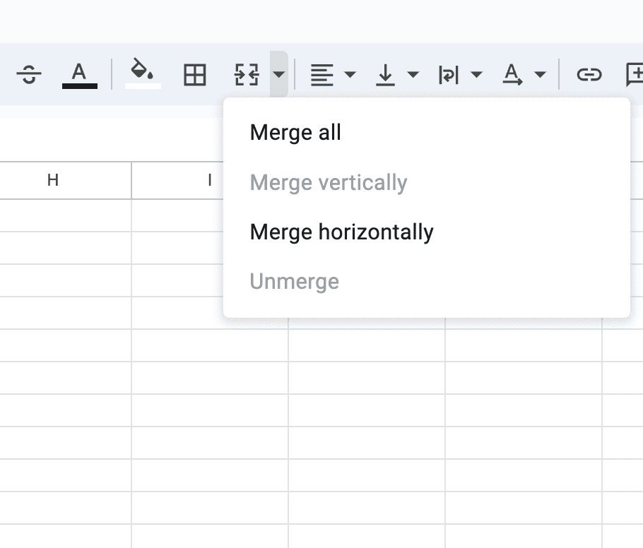
'Merge all' combines all selected cells into one large cell. 'Merge horizontally' merges the cells across rows, while 'Merge vertically' does the same across columns.
Choose the option that best suits your needs.
Step 3: Format the merged cells
After merging cells, you might want to adjust the formatting to make the contents look better. You can align the text (left, center, or right), change the font size, or apply different styles using the formatting options in the toolbar. Remember, merged cells can be formatted just like any other cell in Google Sheets.
How to unmerge cells in Google Sheets?
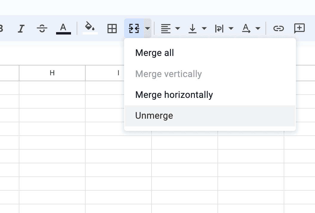
At times, you might need to revert your merged cells back to their original state. To unmerge, simply click on the merged cell, and then click the 'Merge cells' icon in the toolbar. Choose 'Unmerge'. This will divide the merged cell back into its original, individual cells:
How to merge cells in Google Sheets without losing data?
A common concern when merging cells in Google Sheets is the potential loss of data. As mentioned earlier, when cells are merged, Google Sheets retains only the data in the upper-left cell of the selected range, discarding the rest. However, there are ways to merge cells without losing any important information. This section will guide you through the process of merging cells while preserving all your data.
This is how you merge cells in Google Sheets and keep all the data:
Combining data before merging
The key to preserving data lies in combining the contents of the cells before executing the merge. This can be done using a formula. Suppose you have data in cells A1, B1, and C1 that you want to merge into a single cell. Before merging, you can create a formula in another cell (say, D1) that combines the data from these cells. For example, use the formula =A1 & " " & B1 & " " & C1. This formula concatenates the data in A1, B1, and C1, with spaces in between. Adjust the formula as needed for your specific data (such as adding commas or other separators).
Applying the concatenation formula
To apply this formula:
Click on the cell where you want the combined data to appear (e.g., D1).
Enter the formula by typing
=followed by the cell references and the text separators.Press 'Enter', and you will see the combined data from the cells in D1.
Merging cells post-combination
Once you’ve the combined data in one cell, you can proceed with the merging process as described in the earlier sections. Select the range of cells you want to merge, including the cell with the combined data, and use the 'Merge cells' option in the toolbar. Since the combined data is already in the upper-left cell of the range you’re merging, you won't lose any information.
Alternative method: use the 'join text' feature
Another method is to use the 'Join text' feature in Google Sheets. This is particularly useful when dealing with larger ranges or when you need a more dynamic solution:
Select the cells you want to merge.
Right-click and choose 'Format cells'.
Under the 'Text' tab, find the 'Join text' option.
Specify a delimiter, like a comma or space, to separate the text from each cell.
Once configured, the text from all selected cells will be joined in the format you specified, and you can then merge the cells without losing data.
How to merge cells in Google Sheets with a keyboard shortcut?
To merge cells in Google Sheets using a keyboard shortcut, you can follow these steps:
Select the Cells: Click and drag to select the cells you want to merge.
Open the Merge Menu: Press
Alt+Shift+=(on Windows) orOption+Shift+=(on Mac) to open the merge menu.Choose Merge Option: You can then use the arrow keys to navigate to your desired merge option (Merge All, Merge Horizontally, or Merge Vertically) and press
Enterto apply.
Remember, shortcuts can vary based on the operating system and sometimes the version of the software, so if this doesn't work, you might want to check for any updates or variations specific to your setup.
How to merge cells vertically in Google Sheets?
Merging cells vertically in Google Sheets is a straightforward process. Here’s how you do it:
Select the Cells: Click on the first cell you want to merge, and then drag your mouse down to the last cell in the column that you wish to merge. Make sure these cells are aligned vertically.
Merge the Cells:
Using the Menu: Go to the top menu, click on “Format,” then hover over “Merge cells,” and select “Merge vertically.”
Using the Toolbar: You can also find the merge cells icon in the toolbar. It's the icon with two arrows pointing towards each other. After selecting your cells, click on this icon and choose “Merge vertically.”
After completing these steps, the selected cells will be merged into one vertical cell. Remember that if there’s data in any of the cells you're merging, only the upper-left cell's data will be kept; the rest will be deleted.
About the Author

Kris Lachance
Managing Editor
Kris is the Managing Editor of Spreadsheet Secrets. He is a finance professional, writer and entrepreneur based in Canada.
How to Merge Cells in Google Sheets: A Guide
Basics
Apr 30, 2024
We love the fact that Google Sheets has all of these cells. It’s what helps make the data so clear. But what if you want to merge some of those cells together? That’s exactly what this guide covers.
What is cell merging in Google Sheets?
Merging cells involves combining two or more adjacent cells into a single cell. You’ll want to do this when you have data or titles across multiple columns or rows.
Be careful though. When you merge cells, only the upper-left cell will have its data intact. This means that if you have data in the other cells that are being merged, then the data in those cells will be deleted if you merge the cells.
How to merge cells in Google Sheets?
Step 1: Select which cells to merge
First, select the cells you want to merge. You can do this by clicking and dragging your mouse over the cells. For instance, if you want to merge a group of cells from A1 to C1, click on cell A1, hold down your mouse button, and drag across to C1:
Make sure that the cells are next to each other because Google Sheets doesn’t let you merge cells that aren’t next to each other.
Step 2: Merge the cells
Once you’ve selected the cells, it's time to perform the merge. Look for the 'Merge cells' icon in the Google Sheets toolbar. This icon looks like this:
Click on the down arrow to the right of this icon and you’ll see a dropdown menu with three options: 'Merge all', 'Merge horizontally', and 'Merge vertically':
'Merge all' combines all selected cells into one large cell. 'Merge horizontally' merges the cells across rows, while 'Merge vertically' does the same across columns.
Choose the option that best suits your needs.
Step 3: Format the merged cells
After merging cells, you might want to adjust the formatting to make the contents look better. You can align the text (left, center, or right), change the font size, or apply different styles using the formatting options in the toolbar. Remember, merged cells can be formatted just like any other cell in Google Sheets.
How to unmerge cells in Google Sheets?
At times, you might need to revert your merged cells back to their original state. To unmerge, simply click on the merged cell, and then click the 'Merge cells' icon in the toolbar. Choose 'Unmerge'. This will divide the merged cell back into its original, individual cells:
How to merge cells in Google Sheets without losing data?
A common concern when merging cells in Google Sheets is the potential loss of data. As mentioned earlier, when cells are merged, Google Sheets retains only the data in the upper-left cell of the selected range, discarding the rest. However, there are ways to merge cells without losing any important information. This section will guide you through the process of merging cells while preserving all your data.
This is how you merge cells in Google Sheets and keep all the data:
Combining data before merging
The key to preserving data lies in combining the contents of the cells before executing the merge. This can be done using a formula. Suppose you have data in cells A1, B1, and C1 that you want to merge into a single cell. Before merging, you can create a formula in another cell (say, D1) that combines the data from these cells. For example, use the formula =A1 & " " & B1 & " " & C1. This formula concatenates the data in A1, B1, and C1, with spaces in between. Adjust the formula as needed for your specific data (such as adding commas or other separators).
Applying the concatenation formula
To apply this formula:
Click on the cell where you want the combined data to appear (e.g., D1).
Enter the formula by typing
=followed by the cell references and the text separators.Press 'Enter', and you will see the combined data from the cells in D1.
Merging cells post-combination
Once you’ve the combined data in one cell, you can proceed with the merging process as described in the earlier sections. Select the range of cells you want to merge, including the cell with the combined data, and use the 'Merge cells' option in the toolbar. Since the combined data is already in the upper-left cell of the range you’re merging, you won't lose any information.
Alternative method: use the 'join text' feature
Another method is to use the 'Join text' feature in Google Sheets. This is particularly useful when dealing with larger ranges or when you need a more dynamic solution:
Select the cells you want to merge.
Right-click and choose 'Format cells'.
Under the 'Text' tab, find the 'Join text' option.
Specify a delimiter, like a comma or space, to separate the text from each cell.
Once configured, the text from all selected cells will be joined in the format you specified, and you can then merge the cells without losing data.
How to merge cells in Google Sheets with a keyboard shortcut?
To merge cells in Google Sheets using a keyboard shortcut, you can follow these steps:
Select the Cells: Click and drag to select the cells you want to merge.
Open the Merge Menu: Press
Alt+Shift+=(on Windows) orOption+Shift+=(on Mac) to open the merge menu.Choose Merge Option: You can then use the arrow keys to navigate to your desired merge option (Merge All, Merge Horizontally, or Merge Vertically) and press
Enterto apply.
Remember, shortcuts can vary based on the operating system and sometimes the version of the software, so if this doesn't work, you might want to check for any updates or variations specific to your setup.
How to merge cells vertically in Google Sheets?
Merging cells vertically in Google Sheets is a straightforward process. Here’s how you do it:
Select the Cells: Click on the first cell you want to merge, and then drag your mouse down to the last cell in the column that you wish to merge. Make sure these cells are aligned vertically.
Merge the Cells:
Using the Menu: Go to the top menu, click on “Format,” then hover over “Merge cells,” and select “Merge vertically.”
Using the Toolbar: You can also find the merge cells icon in the toolbar. It's the icon with two arrows pointing towards each other. After selecting your cells, click on this icon and choose “Merge vertically.”
After completing these steps, the selected cells will be merged into one vertical cell. Remember that if there’s data in any of the cells you're merging, only the upper-left cell's data will be kept; the rest will be deleted.
About the Author
Kris Lachance
Managing Editor
Kris is the Managing Editor of Spreadsheet Secrets. He is a finance professional, writer and entrepreneur based in Canada.

Spreadsheet Secrets
Helping you get better at all things spreadsheets. From learning functions to helpful tips and tricks. Microsoft Excel, Google Sheets, Apple Numbers, Office 365, whatever you use we can help you with.
Contact us here: ssheetsecrets@gmail.com
© 2024 Spreadsheet Secrets.
Spreadsheet Secrets
Helping you get better at all things spreadsheets. From learning functions to helpful tips and tricks. Microsoft Excel, Google Sheets, Apple Numbers, Office 365, whatever you use we can help you with.
Contact us here: ssheetsecrets@gmail.com
© 2024 Spreadsheet Secrets.
Spreadsheet Secrets
Helping you get better at all things spreadsheets. From learning functions to helpful tips and tricks. Microsoft Excel, Google Sheets, Apple Numbers, Office 365, whatever you use we can help you with.
Contact us here: ssheetsecrets@gmail.com
© 2024 Spreadsheet Secrets.