How to Multiply in Google Sheets: A Guide
Basics
Apr 22, 2024
If you’re using Google Sheets, odds are you will be running some basic math calculations at some point. One of these calculations is multiplication. That’s exactly what this guide covers, so read on if you want to learn how to multiply in Google Sheets.
Introduction to multiplying in Google Sheets
Google Sheets offers a ton functionalities, one of which is the ability to perform basic arithmetic operations like multiplication. Whether you're a student, a business professional, or someone just looking to manage their household expenses, understanding how to multiply in Google Sheets can make you SO much more efficient at managing and working with data.
How to multiply two numbers in Google Sheets?
Let's begin with the simplest form of multiplication in Google Sheets: multiplying two numbers.
For example, maybe you’re asking “what’s 5 times 3” and you want Google Sheets to help you out.
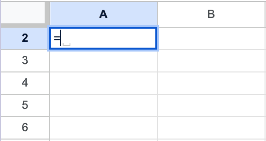
To perform this operation, you need to enter an equal sign (=) in the cell that you want to run the calculation in:
Then, you follow th (=) sign with the numbers that you want to multiply. Separate them with an asterisk (*). For example, to multiply 5 by 3, you would enter =5*3 into a cell. Press Enter, and Google Sheets will display the result, 15, in that cell:
That’s it! As you can see, it’s super easy.
How to multiply cells in Google Sheets?
In most scenarios, especially in data analysis and budgeting, you will need to multiply numbers stored in cells rather than raw numbers.
To multiply two or more cells in Google Sheets, you simply replace the numbers with the respective cell references. Suppose you have a number in cell A1 and another in cell B1, and you wish to multiply these. Click on the cell where you want the result to appear, type =, then click on cell A1, type *, and finally click on cell B1. Now press Enter and you’ll see the result of the multiplication of the contents of cells A1 and B1:

How to multiply multiple cells in Google Sheets?
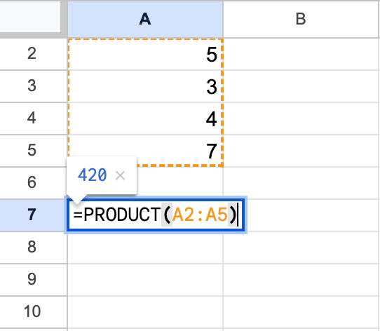
When dealing with more than two numbers, you’ll probably want to use the PRODUCT function. This function multiplies all the numbers given as arguments and returns the product. For instance, if you have numbers in cells A1 through A5 that you want to multiply together, you would enter =PRODUCT(A1:A5) in the cell where you want the result:
This function is particularly useful for multiplying a range of cells, making it a staple in more complex data operations.
How to multiply a cell by a number in Google Sheets?
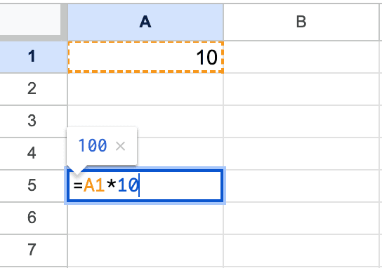
To multiply a cell by a number in Google sheets, you'll first identify the cell containing the number you want to multiply. Let's say this value is in cell A1, and you want to multiply it by 10. Click on the cell where you wish to display the result and type in the formula =A1*10. Upon pressing Enter, Google Sheets calculates the product of the value in cell A1 and 10, displaying the result in the selected cell:
When you copy this formula to other cells, it's important to understand the concept of relative and absolute references in Google Sheets. If you drag the formula down a column or across a row, the cell reference (A1 in our example) will change relatively. This means, if you drag the formula down one row, the formula will change to =A2*10.
If you want to always multiply the value in cell A1 by 10, regardless of where you copy the formula, you should use an absolute reference. You do this by adding dollar signs to the cell reference, like this: =$A$1*10.
If you want to multiply multiple cells by the same number, the process is still straightforward. For instance, if you have values in cells A1 through A5 and wish to multiply each by 10, you can write the formula =A1*10 in cell B1 and then use the fill handle to drag the formula down to B5. Each cell in column B will display the result of the corresponding cell in column A multiplied by 10.
How to multiply columns in Google Sheets?
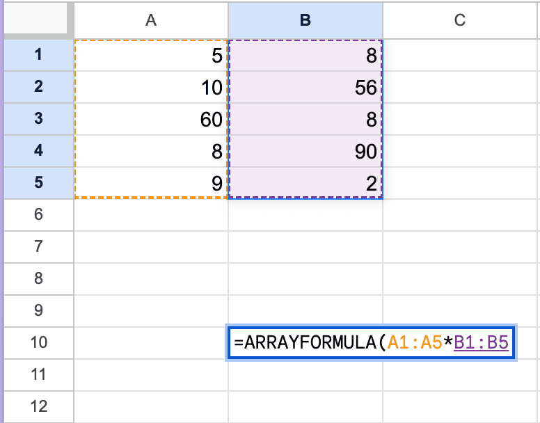
Sometimes, you might need to multiply corresponding entries in two different columns. The best way to do this is using ARRAYFORMULA, which lets you multiply entire columns in one go without the need to drag the fill handle. For instance, if you want to multiply values in column A with column B, you can enter =ARRAYFORMULA(A1:A5*B1:B5) in the first cell of your result column. This will automatically perform the multiplication for each row and display the results in the respective cells:
The array function works great for bulk calculations, which means this same method will work equally well if you want to multiply rows in Google Sheets.
How to multiply 3 numbers in Google Sheets?
To multiply three numbers in Google Sheets, you can use a simple formula. First, select the cell where you want the result to appear. Then, type in = followed by the three numbers you want to multiply, separated by asterisks. For example, if you want to multiply 2, 3, and 4, you would type =2*3*4 into the cell:
Press Enter, and Google Sheets will display the product of these numbers, which is 24, in the selected cell.
How to copy a multiplication formula in Google Sheets?
A common requirement in Google Sheets is replicating a formula across multiple rows or columns. If you've written a multiplication formula in one cell and want to apply it to others, you can use the fill handle. After entering your formula, hover over the bottom right corner of the cell until the cursor turns into a plus sign (+). Click and drag this fill handle to the cells where you want the same operation performed, adjusting cell references accordingly:
How to multiply by a percentage in Google Sheets?
Multiplying by a percentage in Google Sheets is easy. Let's say you want to multiply a number by a percentage. Here are the steps:
Enter the Number and Percentage: First, put your values into the cells. For example, put the number you want to multiply in cell A1 and the percentage in cell B1. Make sure to format the percentage properly by adding the
%symbol, so Google Sheets recognizes it as a percentage. For instance, if you want to multiply by 15%, you should enter15%in cell B1.Use a Formula for Multiplication: In a new cell, use a formula to multiply these two values. The formula would typically look like
=A1*B1. This will automatically handle the percentage calculation.Press Enter: After typing the formula, press Enter. The result of the multiplication will be displayed in the cell where you entered the formula.
For example, If A1 has the value 100 and B1 has the value 15% (ensure it's formatted as a percentage in Google Sheets), then in C1 you’ll enter the formula=A1*B1:
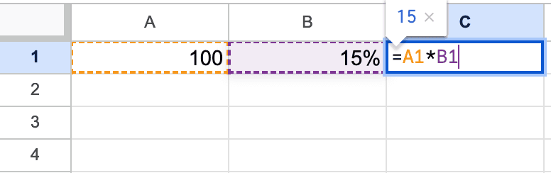
The result that shows up in C1 will be 15, which is 15% of 100.
How to multiply pi in Google Sheets?
To multiply a number by π (pi) in Google Sheets, you can use the PI() function which returns the value of π:
Direct Multiplication: If you want to multiply a specific number by π, you can write a formula like
=A1 * PI(), whereA1is the cell containing the number you want to multiply by π.Multiplying a Range of Numbers: If you have a range of numbers that you want to multiply by π, you can use an array formula or apply the multiplication to each cell individually. For example, if you have numbers in cells ****
A1toA5, you can multiply each by π using a formula like=ARRAYFORMULA(A1:A5 * PI()).Using π in Calculations: You can also use π as part of more complex calculations. For instance, to calculate the area of a circle, you could use a formula like
=PI() * (radius^2), whereradiusis the cell reference or number representing the radius of the circle.
Remember to start your formulas with an equal sign (=), and you can enter these formulas in any cell where you want to see the result.
About the Author

Spreadsheet Secrets
Managing Editor
Kris is the Managing Editor of Spreadsheet Secrets. He is a finance professional, writer and entrepreneur based in Canada.
How to Multiply in Google Sheets: A Guide
Basics
Apr 22, 2024
If you’re using Google Sheets, odds are you will be running some basic math calculations at some point. One of these calculations is multiplication. That’s exactly what this guide covers, so read on if you want to learn how to multiply in Google Sheets.
Introduction to multiplying in Google Sheets
Google Sheets offers a ton functionalities, one of which is the ability to perform basic arithmetic operations like multiplication. Whether you're a student, a business professional, or someone just looking to manage their household expenses, understanding how to multiply in Google Sheets can make you SO much more efficient at managing and working with data.
How to multiply two numbers in Google Sheets?
Let's begin with the simplest form of multiplication in Google Sheets: multiplying two numbers.
For example, maybe you’re asking “what’s 5 times 3” and you want Google Sheets to help you out.
To perform this operation, you need to enter an equal sign (=) in the cell that you want to run the calculation in:
Then, you follow th (=) sign with the numbers that you want to multiply. Separate them with an asterisk (*). For example, to multiply 5 by 3, you would enter =5*3 into a cell. Press Enter, and Google Sheets will display the result, 15, in that cell:
That’s it! As you can see, it’s super easy.
How to multiply cells in Google Sheets?
In most scenarios, especially in data analysis and budgeting, you will need to multiply numbers stored in cells rather than raw numbers.
To multiply two or more cells in Google Sheets, you simply replace the numbers with the respective cell references. Suppose you have a number in cell A1 and another in cell B1, and you wish to multiply these. Click on the cell where you want the result to appear, type =, then click on cell A1, type *, and finally click on cell B1. Now press Enter and you’ll see the result of the multiplication of the contents of cells A1 and B1:
How to multiply multiple cells in Google Sheets?
When dealing with more than two numbers, you’ll probably want to use the PRODUCT function. This function multiplies all the numbers given as arguments and returns the product. For instance, if you have numbers in cells A1 through A5 that you want to multiply together, you would enter =PRODUCT(A1:A5) in the cell where you want the result:
This function is particularly useful for multiplying a range of cells, making it a staple in more complex data operations.
How to multiply a cell by a number in Google Sheets?
To multiply a cell by a number in Google sheets, you'll first identify the cell containing the number you want to multiply. Let's say this value is in cell A1, and you want to multiply it by 10. Click on the cell where you wish to display the result and type in the formula =A1*10. Upon pressing Enter, Google Sheets calculates the product of the value in cell A1 and 10, displaying the result in the selected cell:
When you copy this formula to other cells, it's important to understand the concept of relative and absolute references in Google Sheets. If you drag the formula down a column or across a row, the cell reference (A1 in our example) will change relatively. This means, if you drag the formula down one row, the formula will change to =A2*10.
If you want to always multiply the value in cell A1 by 10, regardless of where you copy the formula, you should use an absolute reference. You do this by adding dollar signs to the cell reference, like this: =$A$1*10.
If you want to multiply multiple cells by the same number, the process is still straightforward. For instance, if you have values in cells A1 through A5 and wish to multiply each by 10, you can write the formula =A1*10 in cell B1 and then use the fill handle to drag the formula down to B5. Each cell in column B will display the result of the corresponding cell in column A multiplied by 10.
How to multiply columns in Google Sheets?
Sometimes, you might need to multiply corresponding entries in two different columns. The best way to do this is using ARRAYFORMULA, which lets you multiply entire columns in one go without the need to drag the fill handle. For instance, if you want to multiply values in column A with column B, you can enter =ARRAYFORMULA(A1:A5*B1:B5) in the first cell of your result column. This will automatically perform the multiplication for each row and display the results in the respective cells:
The array function works great for bulk calculations, which means this same method will work equally well if you want to multiply rows in Google Sheets.
How to multiply 3 numbers in Google Sheets?
To multiply three numbers in Google Sheets, you can use a simple formula. First, select the cell where you want the result to appear. Then, type in = followed by the three numbers you want to multiply, separated by asterisks. For example, if you want to multiply 2, 3, and 4, you would type =2*3*4 into the cell:
Press Enter, and Google Sheets will display the product of these numbers, which is 24, in the selected cell.
How to copy a multiplication formula in Google Sheets?
A common requirement in Google Sheets is replicating a formula across multiple rows or columns. If you've written a multiplication formula in one cell and want to apply it to others, you can use the fill handle. After entering your formula, hover over the bottom right corner of the cell until the cursor turns into a plus sign (+). Click and drag this fill handle to the cells where you want the same operation performed, adjusting cell references accordingly:
How to multiply by a percentage in Google Sheets?
Multiplying by a percentage in Google Sheets is easy. Let's say you want to multiply a number by a percentage. Here are the steps:
Enter the Number and Percentage: First, put your values into the cells. For example, put the number you want to multiply in cell A1 and the percentage in cell B1. Make sure to format the percentage properly by adding the
%symbol, so Google Sheets recognizes it as a percentage. For instance, if you want to multiply by 15%, you should enter15%in cell B1.Use a Formula for Multiplication: In a new cell, use a formula to multiply these two values. The formula would typically look like
=A1*B1. This will automatically handle the percentage calculation.Press Enter: After typing the formula, press Enter. The result of the multiplication will be displayed in the cell where you entered the formula.
For example, If A1 has the value 100 and B1 has the value 15% (ensure it's formatted as a percentage in Google Sheets), then in C1 you’ll enter the formula=A1*B1:
The result that shows up in C1 will be 15, which is 15% of 100.
How to multiply pi in Google Sheets?
To multiply a number by π (pi) in Google Sheets, you can use the PI() function which returns the value of π:
Direct Multiplication: If you want to multiply a specific number by π, you can write a formula like
=A1 * PI(), whereA1is the cell containing the number you want to multiply by π.Multiplying a Range of Numbers: If you have a range of numbers that you want to multiply by π, you can use an array formula or apply the multiplication to each cell individually. For example, if you have numbers in cells ****
A1toA5, you can multiply each by π using a formula like=ARRAYFORMULA(A1:A5 * PI()).Using π in Calculations: You can also use π as part of more complex calculations. For instance, to calculate the area of a circle, you could use a formula like
=PI() * (radius^2), whereradiusis the cell reference or number representing the radius of the circle.
Remember to start your formulas with an equal sign (=), and you can enter these formulas in any cell where you want to see the result.
About the Author
Spreadsheet Secrets
Managing Editor
Kris is the Managing Editor of Spreadsheet Secrets. He is a finance professional, writer and entrepreneur based in Canada.

Spreadsheet Secrets
Helping you get better at all things spreadsheets. From learning functions to helpful tips and tricks. Microsoft Excel, Google Sheets, Apple Numbers, Office 365, whatever you use we can help you with.
Contact us here: ssheetsecrets@gmail.com
© 2024 Spreadsheet Secrets.
Spreadsheet Secrets
Helping you get better at all things spreadsheets. From learning functions to helpful tips and tricks. Microsoft Excel, Google Sheets, Apple Numbers, Office 365, whatever you use we can help you with.
Contact us here: ssheetsecrets@gmail.com
© 2024 Spreadsheet Secrets.
Spreadsheet Secrets
Helping you get better at all things spreadsheets. From learning functions to helpful tips and tricks. Microsoft Excel, Google Sheets, Apple Numbers, Office 365, whatever you use we can help you with.
Contact us here: ssheetsecrets@gmail.com
© 2024 Spreadsheet Secrets.