How to Remove Gridlines in Google Sheets
Formatting
May 2, 2024
This post covers how to get rid of gridlines in Google Sheets.
Removing gridlines in Google Sheets
There are lots of ways you can customize Google Sheets. One of them is to change the look of a sheet - especially the option to remove gridlines. This guide will walk you through all of the steps you need to disable gridlines in Google Sheets, so that your spreadsheet looks as clean as possible.
What are gridlines in Google Sheets?
Gridlines are the faint lines that appear around cells in a spreadsheet to demarcate boundaries between different cells. By default, these gridlines are turned on in Google Sheets to help you track data across the screen. That said, there are case where you might want to remove these gridlines to make the sheet clearer or just generally look prettier.
How to remove gridlines in Google Sheets?
To begin with, open your Google Sheets spreadsheet. Once you have it open in front of you, try to find the ‘View’ menu in the top navigation bar.
Click on the ‘View’ menu to expand it. You’ll see several options listed under it. Look for the ‘Gridlines’ option which is typically accompanied by a checkbox. This checkbox indicates whether the gridlines are currently enabled or disabled. A checked box means gridlines are visible on your sheet, while an unchecked box means they are hidden:
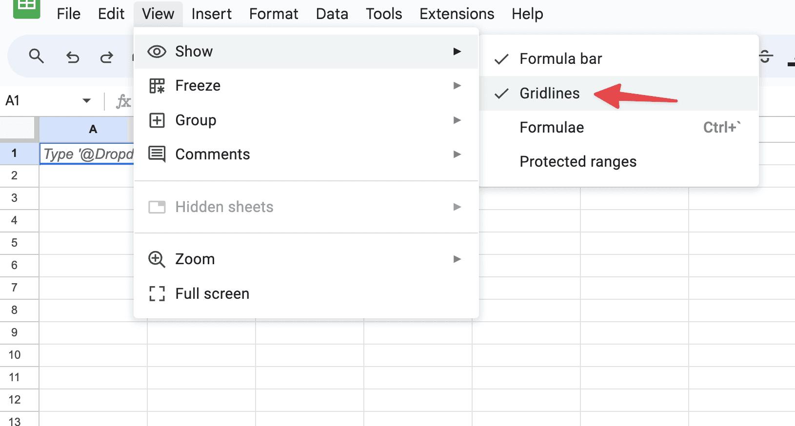
If the ‘Gridlines’ option is checked, all you have to do is click on it to uncheck the box. This action will remove the gridlines from your Google Sheets document, giving you a clean canvas that doesn’t have any cell boundaries.
How to visualize data without gridlines in Google Sheets?
Removing gridlines is super useful when your work involves using Google Sheets to create a presentation or a printable document. Without the clutter of gridlines, your data can stand out more clearly, making it easier for your audience to focus on the content itself rather than the structure of the spreadsheet.
How to restore gridlines in Google Sheets?
If you want to put the gridlines back in, you can do that easily by following the same steps. Go to the ‘View’ menu and click on the ‘Gridlines’ option to check it again. This will bring back the gridlines and help you navigate large sheets more effectively.
How to remove specific gridlines in Google Sheets?
Unfortunately you can’t remove individual gridlines within the main view of a Google Sheets document because gridlines are either all on or all off). But there are ways to visually emphasize or de-emphasize certain cells in your spreadsheet.
This basically means that you’ll have to modify the appearance of certain cells. Gridlines in Google Sheets help delineate the borders of each cell. By default, these lines are uniformly applied across the entire sheet. If you want to "remove" gridlines from specific areas, you essentially have to manipulate the visual aspects of those cells using borders and colors.
How to modify cell appearance in Google Sheets
Adjusting borders
To make certain gridlines appear invisible or emphasize others, adjusting the borders of specific cells is a practical solution. Here’s how you can do it:
Open your Google Sheets document and select the cells where you want to modify the borders.
Right-click on the selected cells to bring up the context menu. From there, choose
Format cells, and thenBorders.Customize your borders. Here you can choose to remove borders (which can mimic the removal of gridlines) or add different styles of borders to highlight specific cells. Use the border tool to erase or add borders as desired:
To simulate the removal of gridlines, select
No bordersfor the selected cells.To emphasize certain cells over others, you might choose a thicker border or a different color.
By carefully applying borders, you can direct attention to specific parts of your sheet effectively, making it appear as if certain gridlines are "removed" by making them blend into the sheet with no delineation.
Use cell background colors
Another way to influence the visibility of gridlines around specific cells is to change the background color:
Select the cells where you want to alter the visual impact of gridlines.
Open the ‘Fill color’ tool from the toolbar (the icon that looks like a paint bucket).
Choose a color that matches the overall background of your sheet (usually white). This makes the gridlines disappear visually for those cells, as the border lines blend with the background color.
Combine both techniques
For even greater control over your sheet's appearance, combine both border adjustments and background color changes. For example, you can remove borders and set the background color to white for a set of cells, making them stand out less, while highlighting others with bold borders.
How to remove bold gridlines in Google Sheets?
Google Sheets doesn’t inherently differentiate between "bold" and "regular" gridlines in the typical sense because all gridlines have a uniform style. However, if certain gridlines appear bolder, it may be due to the presence of custom borders that have been added to the cells. These customized borders can sometimes create the visual effect of having "bold gridlines" around certain cells or blocks of cells.
What’s up with bold gridlines?
The appearance of bold gridlines in Google Sheets usually stems from enhanced cell borders. Users often modify cell borders to organize information visibly or to highlight important data, which can inadvertently create a perception of bold gridlines. To address this, you'll need to adjust or remove these custom borders.
How to remove bold gridlines
Here’s how to effectively remove or modify these bold gridlines by adjusting the borders:
Step 1: Identify the cells
First, open your Google Sheets document and identify the cells or range of cells that are surrounded by what appears to be bold gridlines. Click and drag to select these cells.
Step 2: Access border formatting options
With the cells selected, right-click to open the context menu. From the menu, choose Format cells, then Borders. This will open a border styling menu where you can make adjustments.
Step 3: Remove or adjust borders
In the border menu, you will see options for different types of borders including outer borders, inner borders, and individual border lines (top, bottom, left, right). Here you can:
Remove the borders: If you simply want to remove the bold effect, click on the ‘No borders’ option (often represented by an icon with no lines). This will strip the selected cells of any borders, reverting them to standard gridlines.
Adjust the border style: If you prefer to keep some demarcation but want it to be less prominent, you can choose a lighter color or a thinner style from the border options. Click on the border style icons to adjust them according to your preference.
Step 4: Confirm your changes
After making the desired changes to the borders, click anywhere outside the border menu to close it and see your changes reflected in the sheet. The cells should now integrate more seamlessly with the rest of the grid without bold distinctions.
How to remove gridlines in Google Sheets on an iPad?
Removing gridlines on the iPad version of Google Sheets can be particularly useful when you need a clear and uncluttered view of your data, or when preparing to print a spreadsheet. Here’s how you can do it:
Step 1: Open Google Sheets app on your iPad
First, ensure that you have the Google Sheets app installed on your iPad. Open the app and then select the spreadsheet from which you want to remove the gridlines. If you haven't yet downloaded the app, you can find it in the App Store.
Step 2: Access view options
Once your spreadsheet is open, look at the upper menu of the app. You might need to tap on the screen or the menu button to expand the full menu options if it is not already displayed.
Step 3: Open the "View" menu
In the menu options, find and tap on the “View” option. This might appear as a direct button or be nested inside another menu like "More" depending on your version of the app and your device’s display settings.
Step 4: Toggle off gridlines
Under the "View" settings, you will see an option for “Gridlines.” This will typically have a checkmark next to it if gridlines are currently visible. Tap on “Gridlines” to toggle this option off. When the checkmark disappears, the gridlines will no longer be visible in your spreadsheet.
Additional tips
With gridlines removed, your spreadsheet might look vastly different. Here are a couple of tips to maintain clarity and ease of reading:
Use cell borders: As needed, add borders to specific cells or ranges to define areas clearly without gridlines. This can be done via the cell formatting options.
Adjust column widths and row heights: To improve visibility and organization, adjust the sizes of rows and columns to fit your content appropriately.
About the Author

Kris Lachance
Managing Editor
Kris is the Managing Editor of Spreadsheet Secrets. He is a finance professional, writer and entrepreneur based in Canada.
How to Remove Gridlines in Google Sheets
Formatting
May 2, 2024
This post covers how to get rid of gridlines in Google Sheets.
Removing gridlines in Google Sheets
There are lots of ways you can customize Google Sheets. One of them is to change the look of a sheet - especially the option to remove gridlines. This guide will walk you through all of the steps you need to disable gridlines in Google Sheets, so that your spreadsheet looks as clean as possible.
What are gridlines in Google Sheets?
Gridlines are the faint lines that appear around cells in a spreadsheet to demarcate boundaries between different cells. By default, these gridlines are turned on in Google Sheets to help you track data across the screen. That said, there are case where you might want to remove these gridlines to make the sheet clearer or just generally look prettier.
How to remove gridlines in Google Sheets?
To begin with, open your Google Sheets spreadsheet. Once you have it open in front of you, try to find the ‘View’ menu in the top navigation bar.
Click on the ‘View’ menu to expand it. You’ll see several options listed under it. Look for the ‘Gridlines’ option which is typically accompanied by a checkbox. This checkbox indicates whether the gridlines are currently enabled or disabled. A checked box means gridlines are visible on your sheet, while an unchecked box means they are hidden:
If the ‘Gridlines’ option is checked, all you have to do is click on it to uncheck the box. This action will remove the gridlines from your Google Sheets document, giving you a clean canvas that doesn’t have any cell boundaries.
How to visualize data without gridlines in Google Sheets?
Removing gridlines is super useful when your work involves using Google Sheets to create a presentation or a printable document. Without the clutter of gridlines, your data can stand out more clearly, making it easier for your audience to focus on the content itself rather than the structure of the spreadsheet.
How to restore gridlines in Google Sheets?
If you want to put the gridlines back in, you can do that easily by following the same steps. Go to the ‘View’ menu and click on the ‘Gridlines’ option to check it again. This will bring back the gridlines and help you navigate large sheets more effectively.
How to remove specific gridlines in Google Sheets?
Unfortunately you can’t remove individual gridlines within the main view of a Google Sheets document because gridlines are either all on or all off). But there are ways to visually emphasize or de-emphasize certain cells in your spreadsheet.
This basically means that you’ll have to modify the appearance of certain cells. Gridlines in Google Sheets help delineate the borders of each cell. By default, these lines are uniformly applied across the entire sheet. If you want to "remove" gridlines from specific areas, you essentially have to manipulate the visual aspects of those cells using borders and colors.
How to modify cell appearance in Google Sheets
Adjusting borders
To make certain gridlines appear invisible or emphasize others, adjusting the borders of specific cells is a practical solution. Here’s how you can do it:
Open your Google Sheets document and select the cells where you want to modify the borders.
Right-click on the selected cells to bring up the context menu. From there, choose
Format cells, and thenBorders.Customize your borders. Here you can choose to remove borders (which can mimic the removal of gridlines) or add different styles of borders to highlight specific cells. Use the border tool to erase or add borders as desired:
To simulate the removal of gridlines, select
No bordersfor the selected cells.To emphasize certain cells over others, you might choose a thicker border or a different color.
By carefully applying borders, you can direct attention to specific parts of your sheet effectively, making it appear as if certain gridlines are "removed" by making them blend into the sheet with no delineation.
Use cell background colors
Another way to influence the visibility of gridlines around specific cells is to change the background color:
Select the cells where you want to alter the visual impact of gridlines.
Open the ‘Fill color’ tool from the toolbar (the icon that looks like a paint bucket).
Choose a color that matches the overall background of your sheet (usually white). This makes the gridlines disappear visually for those cells, as the border lines blend with the background color.
Combine both techniques
For even greater control over your sheet's appearance, combine both border adjustments and background color changes. For example, you can remove borders and set the background color to white for a set of cells, making them stand out less, while highlighting others with bold borders.
How to remove bold gridlines in Google Sheets?
Google Sheets doesn’t inherently differentiate between "bold" and "regular" gridlines in the typical sense because all gridlines have a uniform style. However, if certain gridlines appear bolder, it may be due to the presence of custom borders that have been added to the cells. These customized borders can sometimes create the visual effect of having "bold gridlines" around certain cells or blocks of cells.
What’s up with bold gridlines?
The appearance of bold gridlines in Google Sheets usually stems from enhanced cell borders. Users often modify cell borders to organize information visibly or to highlight important data, which can inadvertently create a perception of bold gridlines. To address this, you'll need to adjust or remove these custom borders.
How to remove bold gridlines
Here’s how to effectively remove or modify these bold gridlines by adjusting the borders:
Step 1: Identify the cells
First, open your Google Sheets document and identify the cells or range of cells that are surrounded by what appears to be bold gridlines. Click and drag to select these cells.
Step 2: Access border formatting options
With the cells selected, right-click to open the context menu. From the menu, choose Format cells, then Borders. This will open a border styling menu where you can make adjustments.
Step 3: Remove or adjust borders
In the border menu, you will see options for different types of borders including outer borders, inner borders, and individual border lines (top, bottom, left, right). Here you can:
Remove the borders: If you simply want to remove the bold effect, click on the ‘No borders’ option (often represented by an icon with no lines). This will strip the selected cells of any borders, reverting them to standard gridlines.
Adjust the border style: If you prefer to keep some demarcation but want it to be less prominent, you can choose a lighter color or a thinner style from the border options. Click on the border style icons to adjust them according to your preference.
Step 4: Confirm your changes
After making the desired changes to the borders, click anywhere outside the border menu to close it and see your changes reflected in the sheet. The cells should now integrate more seamlessly with the rest of the grid without bold distinctions.
How to remove gridlines in Google Sheets on an iPad?
Removing gridlines on the iPad version of Google Sheets can be particularly useful when you need a clear and uncluttered view of your data, or when preparing to print a spreadsheet. Here’s how you can do it:
Step 1: Open Google Sheets app on your iPad
First, ensure that you have the Google Sheets app installed on your iPad. Open the app and then select the spreadsheet from which you want to remove the gridlines. If you haven't yet downloaded the app, you can find it in the App Store.
Step 2: Access view options
Once your spreadsheet is open, look at the upper menu of the app. You might need to tap on the screen or the menu button to expand the full menu options if it is not already displayed.
Step 3: Open the "View" menu
In the menu options, find and tap on the “View” option. This might appear as a direct button or be nested inside another menu like "More" depending on your version of the app and your device’s display settings.
Step 4: Toggle off gridlines
Under the "View" settings, you will see an option for “Gridlines.” This will typically have a checkmark next to it if gridlines are currently visible. Tap on “Gridlines” to toggle this option off. When the checkmark disappears, the gridlines will no longer be visible in your spreadsheet.
Additional tips
With gridlines removed, your spreadsheet might look vastly different. Here are a couple of tips to maintain clarity and ease of reading:
Use cell borders: As needed, add borders to specific cells or ranges to define areas clearly without gridlines. This can be done via the cell formatting options.
Adjust column widths and row heights: To improve visibility and organization, adjust the sizes of rows and columns to fit your content appropriately.
About the Author
Kris Lachance
Managing Editor
Kris is the Managing Editor of Spreadsheet Secrets. He is a finance professional, writer and entrepreneur based in Canada.

Spreadsheet Secrets
Helping you get better at all things spreadsheets. From learning functions to helpful tips and tricks. Microsoft Excel, Google Sheets, Apple Numbers, Office 365, whatever you use we can help you with.
Contact us here: ssheetsecrets@gmail.com
© 2024 Spreadsheet Secrets.
Spreadsheet Secrets
Helping you get better at all things spreadsheets. From learning functions to helpful tips and tricks. Microsoft Excel, Google Sheets, Apple Numbers, Office 365, whatever you use we can help you with.
Contact us here: ssheetsecrets@gmail.com
© 2024 Spreadsheet Secrets.
Spreadsheet Secrets
Helping you get better at all things spreadsheets. From learning functions to helpful tips and tricks. Microsoft Excel, Google Sheets, Apple Numbers, Office 365, whatever you use we can help you with.
Contact us here: ssheetsecrets@gmail.com
© 2024 Spreadsheet Secrets.