How to Unhide Rows in Google sheets
Basics
May 1, 2024
There’s probably been one or two times where you’ve been looking for data and noticed that a row is skipped. This usually doesn’t mean that the row was deleted! The most likely explanation is that someone hid the row from view. This is super easy to fix - we’ll cover how to do that in the guide below.
Why rows are hidden sometimes
Google Sheets is a powerful tool for data management and analysis, but sometimes the data you need might be hidden from view. Google Sheets has this feature where you can hide rows to make the spreadsheet more manageable or to focus on specific data.
Imagine you have a Google Sheets document tracking daily sales throughout the month. To focus on a weekly review, you might hide rows containing data for all other weeks, simplifying the view to just the week in question. This makes it easier to analyze and discuss specific weekly trends without the clutter of the entire month's data.
How are rows hidden?
If a row is hidden, that’s usually because someone did so manually. When a row is hidden, it's not deleted or removed; it's simply not visible in the current view of the spreadsheet. The data in the hidden row remains intact and you can still access it once the row is unhidden.
How to unhide a row in Google Sheets?
Step 1: Find the hidden rows
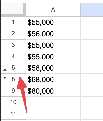
The first step in unhiding rows is to identify where the hidden rows are located in your spreadsheet. You can easily spot the hidden rows by looking at the row numbers on the left side of the sheet. If you notice a break in the sequence of row numbers, it indicates that there are hidden rows. For example, if you see the row numbers jump from 5 to 8, rows 6 and 7 are hidden:
Step 2: Select the rows surrounding the hidden rows
Once you’ve identified the location of the hidden rows, the next step is to select the rows surrounding them. Click on the row number above the hidden rows and drag your mouse to the row number below the hidden rows. For instance, if rows 6 and 7 are hidden, you would click on row 5 and drag down to row 8, thereby selecting rows 5 and 8.
Step 3: Unhide the rows
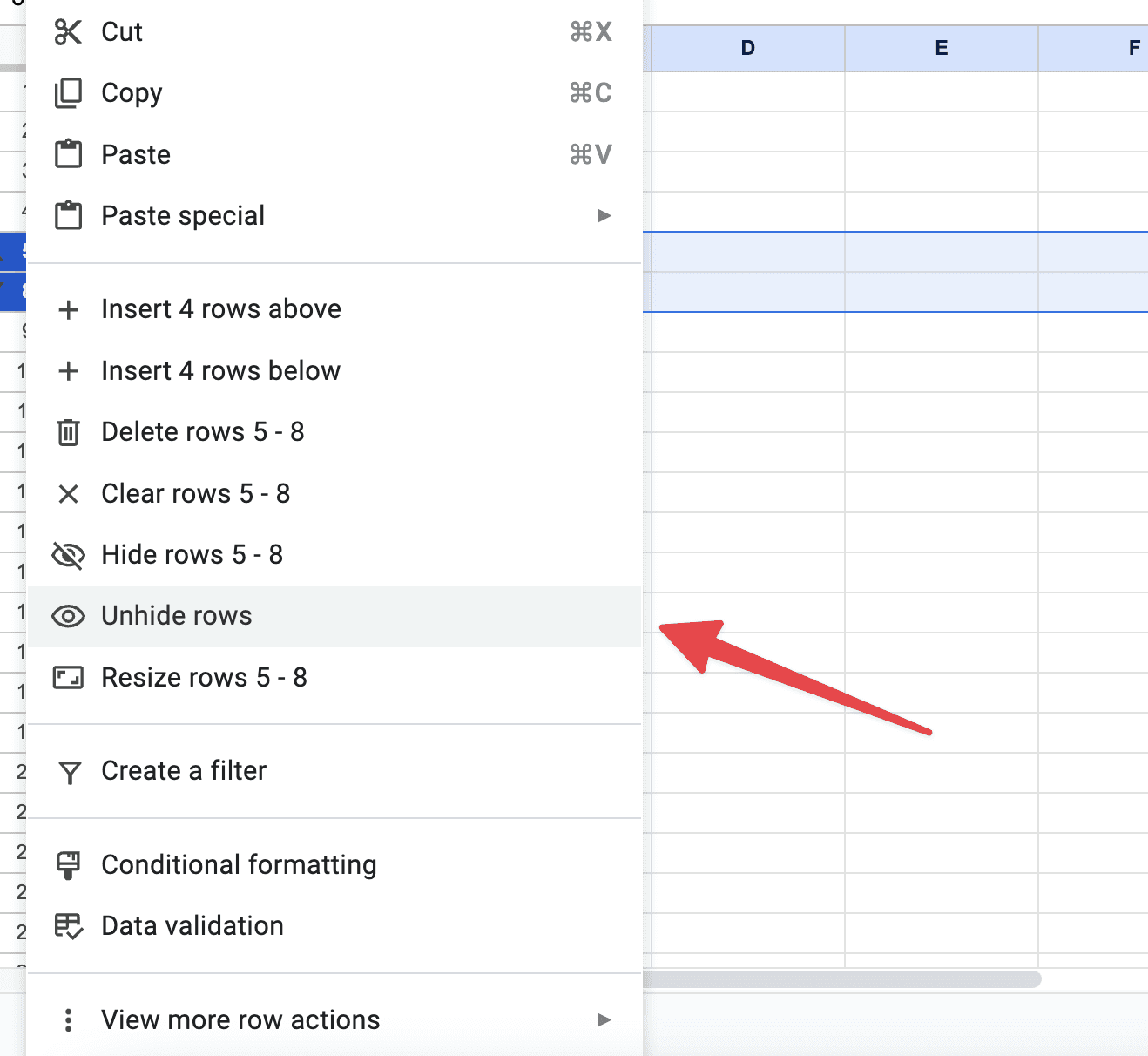
With the surrounding rows selected, you can now proceed to unhide the rows. Right-click on the row numbers (either 5 or 8 in our example) to open a context menu. In this menu, you will find an option labeled "Unhide rows." Click on this option. The hidden rows will immediately become visible on your spreadsheet:
Step 4: Verify the changes
After you’ve unhid the rows, it’s good practice to verify that the correct rows are now visible. Check the sequence of row numbers to ensure that there are no missing numbers and that the previously hidden data is now displayed.
Common issues you might run into
Sometimes you might face issues while trying to unhide rows. If you are unable to unhide rows, there are a few things you can check:
Make sure you are selecting the correct rows surrounding the hidden rows.
If you cannot find the "Unhide rows" option, ensure that you have not selected any cells or columns, as this can change the context menu options.
Verify if you have the necessary permissions to edit the spreadsheet if it's shared with you. Lack of editing permissions can restrict your ability to make changes, including unhiding rows.
How to unhide rows in Google Sheets mobile?
When it comes to unhiding rows in Google Sheets on a mobile device, the process differs slightly from the desktop version due to the constraints and design of mobile interfaces. However, the fundamental concept remains the same.
First, select the row or rows. On a mobile device, the process of selecting rows is slightly different. Tap on the row number just before the hidden rows, and then drag your finger across the screen to the row number just after the hidden rows. For example, if rows 6 and 7 are hidden, you would select rows 5 and 8.
Then you need to access the unhide option. After selecting the rows, tap on the three dots in the top right corner of the screen to bring up the options menu. From this menu, select the ‘Unhide rows’ option. The hidden rows will then become visible in your spreadsheet.
How to unhide rows in Google Sheets on Mac?
The process for Mac is the same as for any platform! Here are some Mac-specific tips though:
Use the Multi-Touch trackpad gestures on your Mac for easier navigation and selection in Google Sheets. For instance, a two-finger scroll can help you navigate through your sheet quickly.
For users with a Magic Mouse, you can use the touch-sensitive surface for smooth scrolling and easy access to the context menu.
Ensure your browser is up to date for optimal compatibility and performance with Google Sheets.
How to unhide all rows in Google Sheets?
There are times when you might need to unhide all the hidden rows in a Google Sheets document: maybe after having hidden several rows across different parts of the sheet for various analyses or presentations. Unhiding all rows at once is a quick way to restore your spreadsheet to its full view. Here’s how:
Open your spreadsheet: Begin by opening your Google Sheets document. Ensure you're working in the correct sheet if your document has multiple sheets.
Select all rows: The key to unhiding all rows simultaneously is to select all the rows in your sheet. You can do this easily by clicking on the grey rectangle located at the top-left corner of your sheet, where the row numbers and column letters intersect. This action selects every cell in your sheet.
Access the unhide option: With all rows selected, right-click anywhere on the row headers (the numbered section on the left) to open the context menu. You may also use the menu at the top: click on 'Format', then hover over 'Row height', and finally, choose 'Unhide rows'.
Unhide all rows: In the context menu, look for the option labeled 'Unhide rows'. It might not be immediately apparent if there are no hidden rows in the selection, but it will be available if you have any hidden rows in your sheet. Click on 'Unhide rows', and all hidden rows across your sheet will be revealed.
Verify the changes: After unhiding, it’s a good practice to scroll through your sheet to ensure that all previously hidden rows are now visible. The row numbers should be sequential without any skips, indicating that all rows are displayed.
About the Author

Kris Lachance
Managing Editor
Kris is the Managing Editor of Spreadsheet Secrets. He is a finance professional, writer and entrepreneur based in Canada.
How to Unhide Rows in Google sheets
Basics
May 1, 2024
There’s probably been one or two times where you’ve been looking for data and noticed that a row is skipped. This usually doesn’t mean that the row was deleted! The most likely explanation is that someone hid the row from view. This is super easy to fix - we’ll cover how to do that in the guide below.
Why rows are hidden sometimes
Google Sheets is a powerful tool for data management and analysis, but sometimes the data you need might be hidden from view. Google Sheets has this feature where you can hide rows to make the spreadsheet more manageable or to focus on specific data.
Imagine you have a Google Sheets document tracking daily sales throughout the month. To focus on a weekly review, you might hide rows containing data for all other weeks, simplifying the view to just the week in question. This makes it easier to analyze and discuss specific weekly trends without the clutter of the entire month's data.
How are rows hidden?
If a row is hidden, that’s usually because someone did so manually. When a row is hidden, it's not deleted or removed; it's simply not visible in the current view of the spreadsheet. The data in the hidden row remains intact and you can still access it once the row is unhidden.
How to unhide a row in Google Sheets?
Step 1: Find the hidden rows
The first step in unhiding rows is to identify where the hidden rows are located in your spreadsheet. You can easily spot the hidden rows by looking at the row numbers on the left side of the sheet. If you notice a break in the sequence of row numbers, it indicates that there are hidden rows. For example, if you see the row numbers jump from 5 to 8, rows 6 and 7 are hidden:
Step 2: Select the rows surrounding the hidden rows
Once you’ve identified the location of the hidden rows, the next step is to select the rows surrounding them. Click on the row number above the hidden rows and drag your mouse to the row number below the hidden rows. For instance, if rows 6 and 7 are hidden, you would click on row 5 and drag down to row 8, thereby selecting rows 5 and 8.
Step 3: Unhide the rows
With the surrounding rows selected, you can now proceed to unhide the rows. Right-click on the row numbers (either 5 or 8 in our example) to open a context menu. In this menu, you will find an option labeled "Unhide rows." Click on this option. The hidden rows will immediately become visible on your spreadsheet:
Step 4: Verify the changes
After you’ve unhid the rows, it’s good practice to verify that the correct rows are now visible. Check the sequence of row numbers to ensure that there are no missing numbers and that the previously hidden data is now displayed.
Common issues you might run into
Sometimes you might face issues while trying to unhide rows. If you are unable to unhide rows, there are a few things you can check:
Make sure you are selecting the correct rows surrounding the hidden rows.
If you cannot find the "Unhide rows" option, ensure that you have not selected any cells or columns, as this can change the context menu options.
Verify if you have the necessary permissions to edit the spreadsheet if it's shared with you. Lack of editing permissions can restrict your ability to make changes, including unhiding rows.
How to unhide rows in Google Sheets mobile?
When it comes to unhiding rows in Google Sheets on a mobile device, the process differs slightly from the desktop version due to the constraints and design of mobile interfaces. However, the fundamental concept remains the same.
First, select the row or rows. On a mobile device, the process of selecting rows is slightly different. Tap on the row number just before the hidden rows, and then drag your finger across the screen to the row number just after the hidden rows. For example, if rows 6 and 7 are hidden, you would select rows 5 and 8.
Then you need to access the unhide option. After selecting the rows, tap on the three dots in the top right corner of the screen to bring up the options menu. From this menu, select the ‘Unhide rows’ option. The hidden rows will then become visible in your spreadsheet.
How to unhide rows in Google Sheets on Mac?
The process for Mac is the same as for any platform! Here are some Mac-specific tips though:
Use the Multi-Touch trackpad gestures on your Mac for easier navigation and selection in Google Sheets. For instance, a two-finger scroll can help you navigate through your sheet quickly.
For users with a Magic Mouse, you can use the touch-sensitive surface for smooth scrolling and easy access to the context menu.
Ensure your browser is up to date for optimal compatibility and performance with Google Sheets.
How to unhide all rows in Google Sheets?
There are times when you might need to unhide all the hidden rows in a Google Sheets document: maybe after having hidden several rows across different parts of the sheet for various analyses or presentations. Unhiding all rows at once is a quick way to restore your spreadsheet to its full view. Here’s how:
Open your spreadsheet: Begin by opening your Google Sheets document. Ensure you're working in the correct sheet if your document has multiple sheets.
Select all rows: The key to unhiding all rows simultaneously is to select all the rows in your sheet. You can do this easily by clicking on the grey rectangle located at the top-left corner of your sheet, where the row numbers and column letters intersect. This action selects every cell in your sheet.
Access the unhide option: With all rows selected, right-click anywhere on the row headers (the numbered section on the left) to open the context menu. You may also use the menu at the top: click on 'Format', then hover over 'Row height', and finally, choose 'Unhide rows'.
Unhide all rows: In the context menu, look for the option labeled 'Unhide rows'. It might not be immediately apparent if there are no hidden rows in the selection, but it will be available if you have any hidden rows in your sheet. Click on 'Unhide rows', and all hidden rows across your sheet will be revealed.
Verify the changes: After unhiding, it’s a good practice to scroll through your sheet to ensure that all previously hidden rows are now visible. The row numbers should be sequential without any skips, indicating that all rows are displayed.
About the Author
Kris Lachance
Managing Editor
Kris is the Managing Editor of Spreadsheet Secrets. He is a finance professional, writer and entrepreneur based in Canada.

Spreadsheet Secrets
Helping you get better at all things spreadsheets. From learning functions to helpful tips and tricks. Microsoft Excel, Google Sheets, Apple Numbers, Office 365, whatever you use we can help you with.
Contact us here: ssheetsecrets@gmail.com
© 2024 Spreadsheet Secrets.
Spreadsheet Secrets
Helping you get better at all things spreadsheets. From learning functions to helpful tips and tricks. Microsoft Excel, Google Sheets, Apple Numbers, Office 365, whatever you use we can help you with.
Contact us here: ssheetsecrets@gmail.com
© 2024 Spreadsheet Secrets.
Spreadsheet Secrets
Helping you get better at all things spreadsheets. From learning functions to helpful tips and tricks. Microsoft Excel, Google Sheets, Apple Numbers, Office 365, whatever you use we can help you with.
Contact us here: ssheetsecrets@gmail.com
© 2024 Spreadsheet Secrets.