Underlining text in Google Sheets is a fundamental skill that can enhance the readability and organization of your data. Whether you're emphasizing key figures, denoting titles, or simply trying to make certain entries stand out, understanding how to underline effectively is essential for anyone using this versatile spreadsheet tool.

Understanding the Basics of Underlining

To start underlining text, you first need to open your Google Sheets document and select the cell or range of cells where you want the underlining to appear. This can be done by clicking on a single cell or by clicking and dragging to select multiple cells.

How to Underline Text in Google Sheets

Applying Underline to Text

Once your cells are selected, you can apply underlining in two primary ways. The quickest method is to just press cmd + u (on Mac) or ctl + u (on PC) on your keyboard.

If you prefer using menus, you can also underline text through the Format menu. Click on 'Format' in the menu bar, then hover over 'Text' and select 'Underline' from the submenu that appears:

This method provides the same result as using the toolbar button, offering an alternative for those who favor menu navigation over direct toolbar interaction.

Customizing Underline Styles

While Google Sheets does not offer as many underline styles as some other text editing programs, it still provides options for basic customization. If you want to change the color or style of your underline, for instance, you will need to explore using cell borders as an alternative to traditional underlining.

To customize using borders, select your cells, then navigate to the 'Borders' icon in the toolbar. This icon typically displays various border options, allowing you to choose a bottom border. By selecting a bottom border, you effectively create a line under your text. You can customize the color and style of this border by choosing from the options presented in the dropdown that appears when you click the borders icon.

How to Get Rid of an Underline in Google Sheets

When working with Google Sheets, you may find the need to remove underlines from your text, whether to clean up the appearance of your data or adjust the formatting for clarity. Removing underlines is as straightforward as applying them, and you can accomplish this task using either the toolbar or the Format menu. Here's how you can efficiently remove underlines from your text in Google Sheets.

Using the Format Menu

You can remove underlines using the Format menu. Start by selecting the cells with the underlined text. Then, click on 'Format' in the top menu bar, hover over 'Text,' and you will see 'Underline' listed among other options. If the text is currently underlined, clicking on 'Underline' will remove the formatting. This method gives you a bit more control and visibility over the formatting options available and is just as effective as using the toolbar.

Removing Custom Underline Styles

If your underline was applied using the borders function as a custom underline style (which might involve a border at the bottom of the cell), removing it follows a similar but slightly adjusted process. First, select the cell or cells where you've applied a bottom border as an underline. Then, click on the 'Borders' icon in the toolbar and look for the option that applies to removing the bottom border (often represented by a line at the bottom of a cell icon with no line). Clicking this will remove the border, effectively removing your custom underline.

Whether you're using the direct underline function or a customized border to underline text, removing this formatting in Google Sheets is straightforward. Both the toolbar and Format menu provide easy-to-use options for toggling off underlines, allowing you to adjust the presentation of your data as needed. Regularly revising and updating your formatting choices, including the use of underlines, ensures that your spreadsheets remain clear, readable, and visually appealing.

Why Would You Want to Underline?

Underlining in spreadsheets like Google Sheets can be a practical and impactful way to draw attention to specific data. A good example of where underlining might be necessary is in financial reporting, specifically within an income statement.

Example: Underlining in an Income Statement

In an income statement, various categories of revenues and expenses are listed to calculate the net income of a business. It's common practice to underline key figures to highlight their importance and to indicate subtotals or totals. For example, you might have different revenue streams like sales revenue, service revenue, and returns or allowances. Below these figures, you’d typically show a subtotal of all revenues, which would be underlined to indicate its significance as a subtotal.

Here's a breakdown of how underlining is used in this context:

1. Subtotals: After listing individual items under revenues and expenses, a subtotal of each category might be underlined. This helps in distinguishing the sum of individual elements from other figures in the list. For instance, if you have multiple lines of revenue, the subtotal of all these revenues is underlined to visually separate it from subsequent expense entries.

2. Final Total: The most important figure in any income statement is the net income, which represents the profit or loss after all revenues and expenses have been accounted for. This figure is typically bolded and underlined, emphasizing its importance as the final takeaway of the document.

3. Visual Hierarchy and Clarity: Underlining serves a functional purpose by creating a clear visual hierarchy. It guides the reader's eye and helps in quickly navigating through the financial figures to understand the financial health of the business.

By using underlining in these ways, the document becomes more organized and easier to interpret, which is crucial for financial documents where precision and clarity are paramount.

TLDR

Underlining text in Google Sheets is a straightforward process that can significantly aid in highlighting important data. Whether through direct underlining or using borders for a more customized approach, these techniques are essential tools in making your spreadsheet both functional and visually appealing. Remember, the key to effective underlining—and spreadsheet management in general—is experimentation and practice, so don't hesitate to try different methods to find what best suits your needs.

Highlighting text in Google Sheets is a fundamental skill that can greatly enhance the readability and organization of your data. Whether you're preparing a report, analyzing data, or simply organizing your information, knowing how to effectively highlight text can make your spreadsheets more visually appealing and easier to navigate. In this guide, we'll explore several methods to highlight text in Google Sheets, including using conditional formatting, manual formatting, and using scripts for more advanced tasks.

How to Highlight Text in a Cell in Google Sheets

Using Conditional Formatting

One of the most powerful tools for highlighting text in Google Sheets is conditional formatting. This feature allows you to automatically apply formatting to cells based on the data they contain. For instance, you can highlight all cells that contain a specific word, number, or meet a certain condition.

To use conditional formatting, start by selecting the range of cells you want to format. Next, navigate to the "Format" menu and choose "Conditional formatting." This opens a sidebar where you can set the rules for when and how text should be highlighted:

You can choose from a variety of conditions such as “Text contains,” “Date is,” “Cell is empty,” and more. After setting your condition, choose a formatting style such as a background color. Once you've configured your settings, click "Done" to apply the formatting.

Manual Text Highlighting

For simpler needs, manual text highlighting is straightforward and quick. Simply select the cells you wish to highlight, then click on the "Fill color" icon in the toolbar, which looks like a paint bucket. Choose your desired color from the dropdown menu to change the background color of the selected cells. This method is ideal for quickly marking important data, categorizing information, or just adding a visual distinction to specific entries.

Advanced Techniques with Google Apps Script

For those who need more customization and control over their text highlighting, Google Apps Script offers a solution. With basic scripting knowledge, you can write custom scripts to automate complex formatting tasks. For example, you can create a script that highlights cells based on multiple conditions or dynamically changes formatting based on external data.

To get started with Google Apps Script, open the "Extensions" menu, select "Apps Script," and start a new project. Here, you can write functions in JavaScript to interact with your Google Sheets data. For highlighting text, you could write a function that loops through rows and applies formatting if certain conditions are met.

What's a Shortcut to Highlight Text in a Google Sheet?

In Google Sheets, there isn't a direct keyboard shortcut to highlight text specifically, but there is a shortcut to open the "Fill color" menu, which you can use to change the background color of selected cells (effectively highlighting them). Here’s how you can do it:

1. Select the cells you want to highlight.

2. Press Alt + Shift + F on Windows or Option + Shift + F on macOS to open the "Fill color" menu.

3. Use the arrow keys to select the color you want and press Enter to apply it.

This sequence allows you to quickly change the background color of cells without reaching for the mouse, thus highlighting your data more efficiently.

What’s a Practical Example?

A practical example of highlighting text in Google Sheets can be seen in managing a project timeline or task list, where different colors are used to indicate the status of various tasks. This helps in quickly assessing the progress of the project at a glance.

Example: Project Timeline Management

Imagine you are managing a project with various tasks, each with different completion statuses like "Not Started", "In Progress", and "Completed". Here’s how you could use highlighting in Google Sheets to manage and visualize this efficiently:

1. Set up your sheet: Organize your sheet with columns for Task Name, Start Date, Due Date, and Status. Fill in each row with the details of different tasks.

2. Apply conditional formatting:

   • Select the column where the status of each task is recorded.

   • Go to the "Format" menu and select "Conditional formatting".

   • Set up three different rules for the statuses:

     • For "Not Started", choose a rule where the text is exactly "Not Started" and set the format to have a red background. This immediately shows that these tasks need attention.

     • For "In Progress", create a rule for text exactly matching "In Progress" and choose a yellow background. This color indicates that the task is underway.

     • For "Completed", set the rule to format cells with the exact text "Completed" with a green background, signaling completion.

3. Update and review: As tasks progress, update the status in the Google Sheet. The colors will automatically change based on the status due to conditional formatting, providing a clear, visual representation of project progress.

By utilizing this method, you create a dynamic, color-coded project timeline that can be easily updated and instantly understood by anyone reviewing the sheet. This helps in maintaining clarity and improving communication among team members or stakeholders regarding the status of project tasks.

What Are Some Things People Like About This Functionality?

The functionality of highlighting text in Google Sheets through conditional formatting and other methods offers numerous benefits that many users appreciate:

1. Visual Clarity: Highlighting helps users quickly discern patterns, trends, and outliers in data. By using different colors to represent different data conditions, users can easily spot what is important, what requires immediate attention, or how things are progressing.

2. Automated Updates: With conditional formatting, the highlights or colors update automatically when the data changes. This is particularly useful in dynamic environments where data entries are frequently modified, as it ensures that the visual cues always reflect the current state of the data without additional manual intervention.

3. Error Reduction: Highlighting can help reduce errors by making incorrect, unusual, or unexpected values stand out. For instance, if a financial spreadsheet is set up to highlight any negative numbers in red, it makes it much easier to catch potentially erroneous entries quickly.

4. Enhanced Productivity: By reducing the time needed to interpret complex data sets, highlighting speeds up data analysis. It makes it easier for users to focus on the right areas, leading to faster decision-making and increased productivity.

5. Customization: Users can tailor highlighting rules to meet specific needs. Whether it’s tracking project milestones, auditing financial records, or managing inventory, conditional formatting can be customized to highlight different statuses, dates, quantities, and more, aligning with the specific requirements of a project or task.

6. Improved Communication: When sharing spreadsheets among team members or presenting data to stakeholders, the use of highlighting makes the information more accessible and understandable to everyone, regardless of their familiarity with the data. This aids in more effective communication and ensures that everyone is on the same page.

7. Data Organization: Highlighting also aids in organizing data by segmenting it visually. This can be particularly useful in large spreadsheets where different sections require distinct visual treatments for easy navigation.

These advantages make text highlighting in Google Sheets a widely used and highly valued feature, particularly in scenarios involving data management, project tracking, and any situation requiring quick and clear data interpretation.

TLDR

Highlighting text in Google Sheets can significantly improve how you present and interact with data. Whether through conditional formatting for dynamic data-driven highlights, manual formatting for quick edits, or custom scripts for tailored solutions, Google Sheets provides a variety of tools to suit any need. By mastering these techniques, you'll be able to create more effective and attractive spreadsheets that better serve your purposes.

Keeping a running total in Google Sheets is a valuable skill for anyone managing data that accumulates over time, such as financial records, inventory counts, or cumulative points in a competition.

A running total is a cumulative sum that updates and increases as new data is added, reflecting the ongoing total amount at each point in a sequence of numbers. It is often used in financial tracking, inventory management, and scoring systems to show progressive totals over time.

This guide will walk you through the process of setting up a running total in a clear and straightforward manner, ensuring you can apply these steps to your own data with ease.

How to Do a Running Total in Google Sheets

Organize your data

First, ensure your data is organized appropriately for tracking a running total. Typically, you will have at least two columns: one for the items or dates (Label) and another for the numbers you want to accumulate (Value). For instance, if you're tracking sales over days, your first column might be the date, and your second column might be the daily sales amount.

Create a running total column

Once your data is set up, you’ll need to create a new column where the running total will be displayed. Let's label this column "Running Total." The key to creating a running total is the use of relative cell references in a formula that adds the current day's value to the total from the previous day.

Writing the Formula

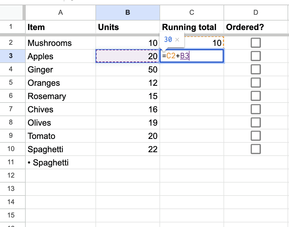
To start the running total, click on the first cell in the "Running Total" column next to your first data entry. Assuming your values are in column B and your running total is in column C, you will enter the following formula in cell C2 (as C1 might be your header):

=B2

This formula sets the initial value of the running total to the first entry in your values column. For the next cell in the running total column (C3), enter the formula:

=C2+B3

This formula adds the value of the second entry (B3) to the previous total (C2):

You will now drag this formula down the column to fill in the rest of the running total. The easiest way to do this is to click on the cell with the formula (C3), and then drag the small square at the bottom-right corner of the cell down through the column to the end of your data:

How to Automatically Create a Running Total

Google Sheets will automatically adjust the formula for each row, so the running total updates as you drag the formula down. Each cell in the "Running Total" column will now add the respective daily value to the cumulative total from the previous cell. This automation ensures that your running total is always up to date with the latest entries.

Verifying and Using Your Data

After setting up your running total, it’s a good practice to verify its accuracy by manually checking the totals for the first few entries. Once confirmed, you can use this running total for various purposes like reports, graphs, or further analysis. For example, you can easily create a line chart to visualize the growth over time using both your daily values and your running total.

How do You Subtract a Running Total in Google Sheets?

To subtract a running total in Google Sheets, you would use a similar approach to creating an additive running total but with subtraction in the formula. For example, if you start with an initial value in cell B2 and you want to subtract subsequent values in column B from this starting point, enter the following formula in cell C2:

=B2

Then, in cell C3, use the formula:

=C2 - B3

Drag this formula down from C3 to the rest of the cells in column C to continue subtracting each new entry in column B from the cumulative total.

What’s a Practical Use Case?

A practical use case for using running totals in Google Sheets can be found in the context of a small business tracking monthly sales and expenses to understand their net income over the year.

Example: Monthly Expense Tracking for a Small Business

Business Name: "Sunshine Tech Solutions"

Scenario: Sunshine Tech Solutions wants to track their monthly operating expenses to manage their budget more effectively and understand their expenditure trends throughout the year.

Data Setup:

• Column A: Month (January, February, March, etc.)

• Column B: Monthly Expenses (values representing each month's expenses)

• Column C: Running Total of Expenses

Application:

• January's Expense in cell B2: $2,000

• Running Total in cell C2 starts with January's expense: =B2 (Output: $2,000)

• February's Expense in cell B3: $1,800

• Running Total for February in cell C3: =C2 + B3 (Output: $3,800)

• The formula in C3 is dragged down through the remaining months.

Usefulness: By December, Sunshine Tech Solutions can see not only each month’s individual expense but also the cumulative total spent over the year. This running total helps in identifying spending trends, planning for future expenses, and preparing financial statements more accurately. For instance, if they notice a consistent increase in the running total, they might consider strategies to cut costs in certain months.

This example demonstrates how running totals can be instrumental in financial planning and management for businesses.

Conclusion

A running total is a simple yet powerful tool in Google Sheets that helps you keep track of cumulative data over time. By following the steps outlined above, you can effectively implement this in your spreadsheets, enhancing your ability to analyze and make decisions based on your data. Whether you are tracking sales, inventory, or any other cumulative data, a running total can provide valuable insights into trends and patterns.

Google Sheets is a versatile tool for organizing data, creating charts, and performing calculations. However, it doesn't natively support bullet points the same way that a word processor would. Fortunately, there are several ways to add bullet points to your Google Sheets, making your lists and data more readable and organized. In this guide, we will explore three methods to add bullet points in Google Sheets: using a custom formula, copying and pasting bullet points, and utilizing the CHAR function.

How to Add Bullet Points in a Cell in Google Sheets

The best way to add bullet points is to use a custom formula. Here’s how:

1. Open your Google Sheets document: Start by opening the Google Sheets document where you want to add bullet points.

2. Select the cell or range of cells: Click on the cell or highlight the range of cells where you want to insert bullet points.

3. Enter the custom formula: In the selected cell, type the following formula: This formula uses the CHAR function to generate a bullet point (the Unicode character for a bullet point is 8226) and concatenates it with the content of cell A1. You can replace "A1" with the reference to the cell you want to add the bullet point to.

   =CHAR(8226)&" "&A10

4. Apply the formula: Press Enter. The cell will now display a bullet point followed by the content of the referenced cell.

Another Way: Copying and Pasting Bullet Points

1. Find a bullet point symbol: Open a text editor or a web browser and search for a bullet point symbol. You can use the following symbol: •

2. Copy the bullet point: Highlight the bullet point symbol and press Ctrl+C (or Cmd+C on Mac) to copy it to your clipboard.

3. Open your Google Sheets document: Navigate to your Google Sheets document.

4. Select the cell or range of cells: Click on the cell or highlight the range of cells where you want to insert bullet points.

5. Paste the bullet point: Double-click the cell to enter edit mode, then press Ctrl+V (or Cmd+V on Mac) to paste the bullet point symbol. You can then type the desired text after the bullet point.

How to Adjust the Appearance of Bullet Points

Once you've added bullet points to your Google Sheets, you may want to adjust their appearance to better suit your needs. Here are a few tips:

• Increase the cell padding: To create more space around the bullet points, increase the cell padding. Click on the cell or range of cells, then go to Format > Number > Custom number format and adjust the padding as needed.

• Change the font size: Adjust the font size to make the bullet points more prominent. Highlight the cells with bullet points, then use the toolbar to increase or decrease the font size.

• Align the text: To align the bullet points with the rest of your text, use the alignment options in the toolbar. You can choose to align the text to the left, center, or right, depending on your preference.

Practical Example

Scenario: Project Task List

Imagine you're a project manager working on a marketing campaign. You need to keep track of tasks assigned to different team members and want to present this information clearly in a Google Sheet. Using bullet points can help differentiate each task and make the list more readable. Here's a practical example:

Scenario: Organizing Marketing Campaign Tasks

Step 1: List the Tasks

You start by listing all the tasks for the campaign in column A of your Google Sheet:

A1: Conduct market research A2: Develop marketing strategy A3: Create content calendar A4: Design promotional materials A5: Launch social media campaign A6: Monitor campaign performance A7: Analyze results and report

Step 2: Add Bullet Points

To make the list more organized, you decide to add bullet points using one of the methods mentioned earlier. Here’s how you can do it using the CHAR function:

1. Select Cell B1: Click on cell B1 where you want to add the first bullet point.

2. Enter the Formula: In cell B1, type the following formula:

   =CHAR(8226)&" Conduct market research"

3. Apply the Formula to Other Cells: Copy the formula in cell B1 and paste it into the subsequent cells (B2, B3, etc.) while changing the task descriptions accordingly:

B1: =CHAR(8226)&" Conduct market research" B2: =CHAR(8226)&" Develop marketing strategy" B3: =CHAR(8226)&" Create content calendar" B4: =CHAR(8226)&" Design promotional materials" B5: =CHAR(8226)&" Launch social media campaign" B6: =CHAR(8226)&" Monitor campaign performance" B7: =CHAR(8226)&" Analyze results and report"

Step 3: Review and Format

After applying the formulas, your sheet will display the tasks with bullet points:

B1: • Conduct market research B2: • Develop marketing strategy B3: • Create content calendar B4: • Design promotional materials B5: • Launch social media campaign B6: • Monitor campaign performance B7: • Analyze results and report

To enhance readability, you can adjust the font size, cell padding, and alignment:

• Increase Cell Padding: Select cells B1 to B7, go to Format > Number > Custom number format, and adjust the padding.

• Change Font Size: Use the toolbar to increase or decrease the font size of the text in cells B1 to B7.

• Align Text: Use the alignment options in the toolbar to ensure the text is neatly aligned.

By adding bullet points to your task list, you make it easier for team members to quickly scan and understand the tasks. This method helps improve organization and communication within the team, ensuring everyone knows their responsibilities and the overall progress of the marketing campaign. This approach can be applied to various other scenarios, such as creating shopping lists, event planning checklists, or any other list where clear organization is beneficial.

Conclusion

Adding bullet points in Google Sheets enhances the readability and organization of your data. By using a custom formula, copying and pasting bullet points, or utilizing the CHAR function, you can easily incorporate bullet points into your spreadsheets. Experiment with these methods to find the one that best suits your workflow, and make your Google Sheets more effective and visually appealing.